Some non-convex quadratic models I
The new version of Gurobi v 9 introduced support for non-convex quadratic models. Cplex already supported some classes of such models (such as non-convex QPs). Here are just some models we can now try to solve with these solvers.
It is noted that you need to specify a solver option for Cplex and Gurobi to accept most non-convex models, Some models can be reformulated by the solver, but "real" con-convex models require the option OptimalityTarget 3 (Cplex) or NonConvex 2 (Gurobi).
It is noted that you need to specify a solver option for Cplex and Gurobi to accept most non-convex models, Some models can be reformulated by the solver, but "real" con-convex models require the option OptimalityTarget 3 (Cplex) or NonConvex 2 (Gurobi).
1a. Largest Empty Rectangle
Given is an area with \(n\) points:
The problem is to find the largest empty rectangle, i.e., without any points inside. The solution looks like:
The idea behind the model below, it that a data point \(p_i\) must be either left, right, below or above the rectangle. So it the coordinates of the rectangle are denoted by \(r_{x,lo},r_{x,up},r_{y_lo},r_{y_up}\), then at least one of the following constraints must hold: \[\begin{align} & p_{i,x} \le r_{x,lo} \\& p_{i,y} \le r_{y,lo} \\ & p_{i,x} \ge r_{x,up} \\& p_{i,y} \ge r_{y,up}\end{align}\] The complete mathematical model to find this rectangle can be stated as:
For the 2d case, the objective can be written as \[\min\> \mathit{area} = (r_{x,up}-r_{x,lo})\cdot (r_{y,up}-r_{y,lo})\] The outer area is a given rectangle with limits \(L_x, U_x, L_y, U_x\). I used here the unit box: \(L_x=L_y = 0\) and \(U_x=U_y = 1\). The big-M constants \(M_x, M_y\) need tight values. We can use the area dimensions for that. For a formulation without big-M constraints, we can implement implications using indicator constraints: \[\begin{align} & \delta_{i,c,lo}=1 \implies p_{i,c} \le r_{i,c,lo} \\ &\delta_{i,c,up}=1 \implies p_{i,c} \ge r_{i,c,up}\end{align}\]
The problem is not convex because of the objective. It is noted that we can simplify the objective a bit by writing \[\begin{align}\max\>&\mathit{area} = \mathit{side}_x \cdot \mathit{side}_y\\ & \mathit{side}_c = r_{c,up} - r_{c,lo}\end{align}\] This is a small problem with just 4 continuous quadratic variables and \(n\times 4\) binary variables. Gurobi or Cplex solve this model very quickly.
This problem can also be solved with available global solvers. Both Antigone and Baron have no problems with it. The optimal solution looks like:
I also tried the open-source solver Couenne. That was a surprise:
This is obviously a bad and non-optimal solution. I don't know what is going on here, but this looks like a bug.
It is easy to make a 3d version of the model above. Just replace \(c = \{x,y\}\) by \(c = \{x,y,z\}\). Unfortunately, there is one complication: now the model has an objective that is no longer quadratic. However, this can be fixed by chaining: \[\begin{align} \max\>&\mathit{volume} = \mathit{area}\cdot \mathit{side}_{z}\\ & \mathit{area} = \mathit{side}_{x} \cdot \mathit{side}_{y} \\ & \mathit{side}_c = r_{c,up}-r_{c,lo} && \forall c \end{align}\]
A solution can look like:
Note that Cplex can not handle this problem: Cplex allows non-convexities in the objective only (apart for some cases where it can reformulate things).
Here \(i\) indicates the point, \(i \in \{1,\dots,n\}\) and \(c\) is the coordinate. For a 2D problem, we have \(c \in \{x,y\}\).
When we use \(n=50\) random points, Gurobi is not able to even come close to proven optimality, I used a time limit of 2 hours, and the final gap is enormous:
Summary:
The big gap is partly due to the small best-found solution (0.01935). But mainly: this is a very difficult job for Gurobi. Even when the problem is relatively small: just 100 continuous variables,
By inspecting the solution, we see this solution is not very good at all:
I expect a much more regular pattern.
We can try to improve performance by noticing there is much symmetry in the model. The same solution can be obtained by just renumbering the points. To break symmetry, I added the constraint: \[\sum_c x_{i,c} \ge \sum_c x_{i-1,c}\] This was not very successful:
 |
| n=50 random points |
The problem is to find the largest empty rectangle, i.e., without any points inside. The solution looks like:
 |
| Largest empty rectangle |
The idea behind the model below, it that a data point \(p_i\) must be either left, right, below or above the rectangle. So it the coordinates of the rectangle are denoted by \(r_{x,lo},r_{x,up},r_{y_lo},r_{y_up}\), then at least one of the following constraints must hold: \[\begin{align} & p_{i,x} \le r_{x,lo} \\& p_{i,y} \le r_{y,lo} \\ & p_{i,x} \ge r_{x,up} \\& p_{i,y} \ge r_{y,up}\end{align}\] The complete mathematical model to find this rectangle can be stated as:
| Smallest empty rectangle |
|---|
| \[\begin{align} \max\> & \color{darkred}{\mathit{area}} = \prod_c (\color{darkred}r_{c,up}-\color{darkred}r_{c,lo}) \\ & \color{darkblue}p_{i,c} \le \color{darkred}r_{c,lo}+\color{darkblue}M_c(1-\color{darkred}\delta_{i,c,lo}) && \forall i,c\\ & \color{darkblue}p_{i,c} \ge \color{darkred}r_{c,up}-\color{darkblue}M_c(1-\color{darkred}\delta_{i,c,up}) && \forall i,c\\ & \sum_{c,s} \color{darkred}\delta_{i,c,s} \ge 1 && \forall i \\ & \color{darkblue} L_c \le \color{darkred}r_{c,lo} \le \color{darkred}r_{c,up}\le \color{darkblue} U_c \\ & \color{darkred}\delta_{i,c,s} \in \{0,1\} \end{align} \] |
| \[\begin{align} & i = \{1,\dots,n\}\\ & c = \{x,y\}\\ & s = \{lo,up\} \\ & \color{darkblue} L_c = 0 \\ & \color{darkblue} U_c = 1 \\ & \color{darkblue} M_c = \color{darkblue}U_c-\color{darkblue}L_c \end{align}\] |
For the 2d case, the objective can be written as \[\min\> \mathit{area} = (r_{x,up}-r_{x,lo})\cdot (r_{y,up}-r_{y,lo})\] The outer area is a given rectangle with limits \(L_x, U_x, L_y, U_x\). I used here the unit box: \(L_x=L_y = 0\) and \(U_x=U_y = 1\). The big-M constants \(M_x, M_y\) need tight values. We can use the area dimensions for that. For a formulation without big-M constraints, we can implement implications using indicator constraints: \[\begin{align} & \delta_{i,c,lo}=1 \implies p_{i,c} \le r_{i,c,lo} \\ &\delta_{i,c,up}=1 \implies p_{i,c} \ge r_{i,c,up}\end{align}\]
The problem is not convex because of the objective. It is noted that we can simplify the objective a bit by writing \[\begin{align}\max\>&\mathit{area} = \mathit{side}_x \cdot \mathit{side}_y\\ & \mathit{side}_c = r_{c,up} - r_{c,lo}\end{align}\] This is a small problem with just 4 continuous quadratic variables and \(n\times 4\) binary variables. Gurobi or Cplex solve this model very quickly.
This problem can also be solved with available global solvers. Both Antigone and Baron have no problems with it. The optimal solution looks like:
----     50 VARIABLE area.L                =        0.113

----     50 VARIABLE r.L  coordinates of rectangle

           lo          up

x       0.403       0.792
y       0.285       0.575
I also tried the open-source solver Couenne. That was a surprise:
               S O L V E      S U M M A R Y

     MODEL   m                   OBJECTIVE  area
     TYPE    MIQCP               DIRECTION  MAXIMIZE
     SOLVER  COUENNE             FROM LINE  49

**** SOLVER STATUS     1 Normal Completion
**** MODEL STATUS      1 Optimal
**** OBJECTIVE VALUE                0.0121


----     50 VARIABLE area.L                =        0.012

----     50 VARIABLE r.L  coordinates of rectangle

           lo          up

x       0.939       0.982
y       0.720       1.000
This is obviously a bad and non-optimal solution. I don't know what is going on here, but this looks like a bug.
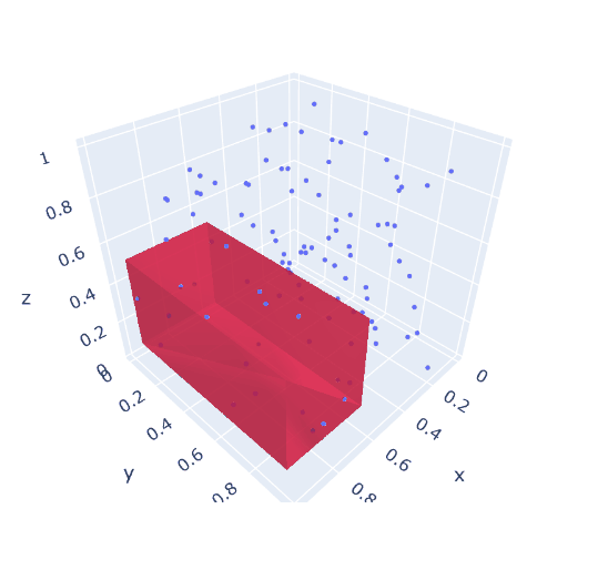
1b. 3d largest box
It is easy to make a 3d version of the model above. Just replace \(c = \{x,y\}\) by \(c = \{x,y,z\}\). Unfortunately, there is one complication: now the model has an objective that is no longer quadratic. However, this can be fixed by chaining: \[\begin{align} \max\>&\mathit{volume} = \mathit{area}\cdot \mathit{side}_{z}\\ & \mathit{area} = \mathit{side}_{x} \cdot \mathit{side}_{y} \\ & \mathit{side}_c = r_{c,up}-r_{c,lo} && \forall c \end{align}\]
A solution can look like:
----     52 VARIABLE area.L                =        0.340
            VARIABLE volume.L              =        0.146

----     52 VARIABLE r.L  coordinates of 3D box

           lo          up

x       0.608       0.998
y       0.091       0.963
z       0.140       0.571
Note that Cplex can not handle this problem: Cplex allows non-convexities in the objective only (apart for some cases where it can reformulate things).
 |
| 3d version: largest box not clashing with given points |
2. Hostile Brothers Problem
A father is facing the following problem. He has has a plot of land. And he has \(n\) sons, who don't get along at all. In order to minimize friction, he wants to build a house for each of his sons, such that the minimum distance between them is maximized. The mathematical model can look like:
| Hostile Brothers Problem |
|---|
| \[\begin{align} \max\> & \color{darkred}z \\ & \color{darkred}z \le \sum_{c} (\color{darkred}x_{i,c}-\color{darkred}x_{j,c})^2&& \forall i\lt j\\ & \color{darkred}x_{i,c} \in [\color{darkblue}L,\color{darkblue}U]\end{align} \] |
Here \(i\) indicates the point, \(i \in \{1,\dots,n\}\) and \(c\) is the coordinate. For a 2D problem, we have \(c \in \{x,y\}\).
When we use \(n=50\) random points, Gurobi is not able to even come close to proven optimality, I used a time limit of 2 hours, and the final gap is enormous:
 1560307 1354785    0.40487   42 1653    0.01935    0.67173  3371%   332 7171s
 1562085 1356368     cutoff  283         0.01935    0.67173  3371%   332 7177s
 1563023 1356980     cutoff  285         0.01935    0.67173  3371%   332 7180s
 1564565 1358071    0.01937  248  930    0.01935    0.67173  3371%   332 7190s
 1565720 1359205    0.60071   48 1510    0.01935    0.67173  3371%   332 7196s
 1567335 1359826     cutoff  272         0.01935    0.67173  3371%   332 7200s


Cutting planes:
  RLT: 1312

Explored 1567341 nodes (520860935 simplex iterations) in 7200.00 seconds
Thread count was 8 (of 16 available processors)
Summary:
- Best found solution: 0.01935
- Best possible objective value: 0.6173
- Relative gap: 3371%
The big gap is partly due to the small best-found solution (0.01935). But mainly: this is a very difficult job for Gurobi. Even when the problem is relatively small: just 100 continuous variables,
By inspecting the solution, we see this solution is not very good at all:
 |
| Solution found by Gurobi after 2 hours (obj=0.01935) |
I expect a much more regular pattern.
We can try to improve performance by noticing there is much symmetry in the model. The same solution can be obtained by just renumbering the points. To break symmetry, I added the constraint: \[\sum_c x_{i,c} \ge \sum_c x_{i-1,c}\] This was not very successful:
 2978972 2407171    0.01708  130  813    0.00885    0.64271  7159%   222 7180s
 2981109 2409232    0.52720   64 2378    0.00885    0.64271  7159%   222 7185s
 2984648 2411500    0.20399  107 2156    0.00885    0.64271  7159%   222 7191s
 2986302 2412811    0.12220  127 1721    0.00885    0.64271  7159%   222 7195s
 2987852 2413879    0.06942  175 1728    0.00885    0.64271  7159%   222 7200s

Explored 2988184 nodes (662244035 simplex iterations) in 7200.01 seconds
Thread count was 8 (of 16 available processors)
So we see:
- The best-found solution (0.00885) is worse than before (0.01935)
- The best possible solution (0.64271) is worse than before (0.6173)
- The relative gap is worse (7159% vs 3371%)
As an alternative, let's try Baron on this model. I dropped the symmetry breaking constraint here (adding this constraint was not beneficial, at least not during the initial period of the search). We see in the first few minutes:
  Iteration    Open nodes         Time (s)    Lower bound      Upper bound
*         1             1             5.51     0.257746E-01     2.00000
*         1             1             7.22     0.274782E-01     2.00000
          1             1             7.41     0.274782E-01     2.00000
         12             7            49.51     0.274782E-01     1.72727
         31            16            80.03     0.274782E-01     1.72727
         46            24           111.27     0.274782E-01     1.72727
I.e. Baron finds a much better solution very quickly (but is far from getting the gap close to zero).
Another approach is to use a multi-start approach with a local NLP solver. Generate a random starting point, solve, and repeat. When I do this 20, I see when I use the CONOPT NLP solver:
Another approach is to use a multi-start approach with a local NLP solver. Generate a random starting point, solve, and repeat. When I do this 20, I see when I use the CONOPT NLP solver:
----     57 PARAMETER objs  objective values of NLP solver

cycle1  0.02751,    cycle2  0.02669,    cycle3  0.02705,    cycle4  0.02041,    cycle5  0.02620,    cycle6  0.01235
cycle7  0.02675,    cycle8  0.02590,    cycle9  0.02660,    cycle10 0.02679,    cycle11 0.02558,    cycle12 0.02644
cycle13 0.02622,    cycle14 0.02625,    cycle15 0.02620,    cycle16 0.02749,    cycle17 0.02742,    cycle18 0.02692
cycle19 0.02675,    cycle20 0.02688,    best    0.02751
This is the best we have seen so far. By accident, the best results were found in the first cycle. The results look like:
 |
| Best solution with Multi-start Conopt (obj=0.02751) |
This solution looks much better than the one Gurobi found. In addition, CONOPT needs only 30 seconds to solve these 20 problems.
Conclusion:
- Cplex cannot solve this problem
- Gurobi finds a solution with objective 0.01935 (time limit: 2 hours)
- Baron finds a solution of 0.02748 in 100 seconds
- Conopt finds a solution of 0.02751 in a loop of 20 solves that takes 30 seconds
- Increasing this to 200 solves gives an objective of 0.02771
- Remember that we are maximizing
Even though this is a non-convex quadratic problem, it makes sense to look beyond quadratic solvers.


