Tuesday, November 27, 2018

Chess and solution pool

The \(n\)-queens problem is a popular example of a "chessboard non-attacking problem" [1,2]:

  • On an \(n \times n\) chessboard place as many queens as possible such that none of them is attacked
  • Given this, how many different ways can we place those queens?

We use the usual \(8 \times 8\) board.

Rooks


A related, simpler problem is about placing rooks. The optimization problem is very simple: it is an assignment problem:


n-Rooks Problem
\[\begin{align}\max&\> \color{DarkRed}z=\sum_{i,j} \color{DarkRed} x_{i,j}\\ & \sum_j \color{DarkRed}x_{i,j} \le 1 && \forall i\\& \sum_i \color{DarkRed}x_{i,j} \le 1 && \forall j\\ & \color{DarkRed}x_{i,j}\in\{0,1\} \end{align}\]

For an \(8 \times 8\) board it is obvious that the number of rooks we can place is 8. Here we show two configurations:


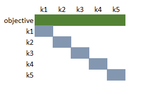
We can easily answer: how many alternative configuration with 8 rooks can we find? This is \[n! = 8! = 40,320\] Basically, we enumerate all row and column permutations of the diagonal depicted above. We can use the solution pool in solvers like Cplex and Gurobi to find all of them. Here I use Cplex and the performance is phenomenal: all 40,320 solutions are found in 16 seconds.

Board


In the models in this write-up, I assume a board that has the coordinates:

Coordinate System in Models

This also means that the diagonals:
Main diagonal and anti-diagonal

have the form \(\{(i,j)|i=j\}\) and \(\{(i,j)|i+j=9\}\). More generally, for the downward sloping main diagonals we have the rule: \[i=j+k\] for \(k=-6,\dots,6\). The anti-diagonals can be described as: \[i+j=k\] for \(k=3,\dots,15\). We can illustrate this with:

Diagonals and anti-diagonals


The first picture has cell values \(a_{i,j}=i-j\) and the second one has cell values \(a_{i,j}=i+j\).


Bishops


The model for placing bishops is slightly more complicated: we need to check the main diagonals and the anti-diagonals. We use the notation from the previous paragraph. So with this, our model can look like:

n-Bishops Problem
\[\begin{align}\max& \>\color{DarkRed}z=\sum_{i,j} \color{DarkRed} x_{i,j}\\ & \sum_{i-j=k} \color{DarkRed}x_{i,j} \le 1 && k=-(n-2),\dots,(n-2)\\& \sum_{i+j=k} \color{DarkRed}x_{i,j} \le 1 && k=3,\dots,2n-1\\ & \color{DarkRed}x_{i,j}\in\{0,1\} \end{align}\]

Note that these constraints translate directly into GAMS:

bishop_main(k1).. sum((i,j)$(v(i)-v(j)=v(k1)),x(i,j)) =l= 1;
bishop_anti(k2).. sum((i,j)$(v(i)+v(j)=v(k2)),x(i,j)) =l= 1;

Two possible solutions are:

We can accommodate 14 bishops. There are 256 different solutions (according to Cplex).

Note: the GAMS display of the solution is not so useful:


----     47 VARIABLE x.L  

            1           2           4           5           7           8

1           1                       1           1           1
2           1
3           1                                                           1
6           1                                                           1
7                                                                       1
8           1           1           1           1

For this reason I show the solution using the \(\LaTeX\) chessboard package [5]. You should be aware that the coordinate system is different than what we use in the models.

Queens


The \(n\) queens problem is now very simple: we just need to combine the two previous models.

n-Queens Problem
\[\begin{align}\max&\> \color{DarkRed}z= \sum_{i,j} \color{DarkRed} x_{i,j}\\ & \sum_j \color{DarkRed}x_{i,j} \le 1 && \forall i\\& \sum_i \color{DarkRed}x_{i,j} \le 1 && \forall j\\ & \sum_{i-j=k} \color{DarkRed}x_{i,j} \le 1 && k=-(n-2),\dots,(n-2)\\& \sum_{i+j=k} \color{DarkRed}x_{i,j} \le 1 && k=3,\dots,2n-1\\ & \color{DarkRed}x_{i,j}\in\{0,1\} \end{align}\]

A solution can look like:

We can place 8 queens and there are 92 solutions.

Notes:

  • Cplex delivered 91 solutions. This seems to be a tolerance issue. I used a solution pool absolute gap of zero (option SolnPoolAGap=0 or as it is called recently: mip.pool.absgap=0) [4]. As the objective jumps by one, it is safe to set the absolute gap to 0.01. With this gap we found all 92 solutions. Is this a bug? Maybe. Possibly. Probably. This 92-th solution is not supposed to be cut off. Obviously, poor scaling is not an issue here: this model is as well-scaled as you can get. I suspect that the (somewhat poorly understood) combination of tolerances (feasibility, integer, optimality) causes Cplex to behave this way. If too many binary variables assume 0.99999 (say within the integer tolerance) we have an objective which is too small. Indeed, we can also get to 92 solutions by setting the integer tolerance epint=0.  Note that setting the integer tolerance to zero will often increase solution times.
    Often tolerances "help" us: they make it easier to find feasible or optimal solutions. Here is a case when they really cause problems.
    Of course this discussion is not a good advertisement for Mixed Integer Programming models. Preferably we should not have to worry about technical details such as tolerances when building and solving models that are otherwise fairly straightforward (no big-M's, well-scaled, small in size).
  • A two step algorithm can help to prevent the tolerance issue discussed above:
    1. Solve the maximization problem: we find max number of queens \(z^*\).
    2. Create a feasibility problem with number of queens equal to \(z^*\). I.e. we add the constraint: \[\sum_{i,j} x_{i,j}=z^*\] This problem has no objective. Find all feasible integer solutions using the solution pool. We don't need to set a solution pool gap for this.
    On the surface, this looks just like the method above. However, physically having the constraint \(\sum x_{i,j}=z^*\) in the model will make sure all relaxations obey this constraints. So any binary variables that are automatically integer (i.e. close to 0 or 1) will never cause us to deviate too much from \(z^*\). This is subtle.
  • Many of the 92 solutions are the result of simple symmetric operations, such as rotating the board, or reflection [2]. The number of different solutions after ignoring these symmetries is just 12. The GAMS model in [3] finds those.
  • The model in [3] handles the bishop constraints differently, by calculating an offset and writing \[\sum_i x_{i,i +\mathit{sh}_s} \le 1 \>\>\forall s\] I somewhat prefer our approach.  

Kings


Kings are handled quite cleverly in [1]. They observe that there cannot be more than one king in each block \[\begin{matrix} x_{i,j} & x_{i,j+1}\\ x_{i+1,j} & x_{i+1,j+1}\end{matrix}\] Note that we only have to look forward (and downward) as a previous block would have covered things to the left (or above). The model can look like:

n-Kings Problem
\[\begin{align}\max& \>\color{DarkRed}z=\sum_{i,j} \color{DarkRed} x_{i,j}\\ & \color{DarkRed}x_{i,j}+\color{DarkRed}x_{i+1,j}+\color{DarkRed}x_{i,j+1}+\color{DarkRed}x_{i+1,j+1}\le 1 && \forall i,j\le n-1\\ & \color{DarkRed}x_{i,j}\in\{0,1\} \end{align}\]

Two solutions are:


We can place 16 kings, and there are a lot of possible configurations: 281,571 (says Cplex).

Knights


To place knights we set up a set \(\mathit{jump}_{i,j,i',j'}\) indicating if we can jump from cell \((i,j)\) to cell \((i',j')\). We only need to look forward, so for each \((i,j)\) we need to consider four cases:
\(j\)\(j+1\)\(j+2\)
\(i-2\)\(x_{i-2,j+1}\)
\(i-1\)\(x_{i-1,j+2}\)
\(i\)\(x_{i,j}\)
\(i+1\)\(x_{i+1,j+2}\)
\(i+2\)\(x_{i+2,j+1}\)

Note that near the border we may have fewer than four cases. In GAMS we can populate the set \(\mathit{jump}\) straightforwardly:

jump(i,j,i-2,j+1) = yes;
jump(i,j,i-1,j+2) = yes;
jump(i,j,i+1,j+2) = yes;
jump(i,j,i+2,j+1) = yes;

The model can look like:

n-Knights Problem
\[\begin{align}\max& \>\color{DarkRed}z=\sum_{i,j} \color{DarkRed} x_{i,j}\\ & \color{DarkRed}x_{i,j}+\color{DarkRed}x_{i',j'}\le 1 && \forall i,j,i',j'|\mathit{jump}_{i,j,i',j'}\\ & \color{DarkRed}x_{i,j}\in\{0,1\} \end{align}\]


We can place 32 knights. There are only two different solutions:


Conclusion


The solution pool is a powerful tool to enumerate possibly large numbers of integer solutions. However, with default tolerances, setting the solution pool absolute gap tolerance to zero may cause perfectly good integer solutions to be missed. This is dicey stuff.

References

  1. L. R. Foulds and D. G. Johnston, An Application of Graph Theory and Integer Programming: Chessboard Non-Attacking Puzzles, Mathematics Magazine Vol. 57, No. 2 (Mar., 1984), pp. 95-104
  2. Eight queens puzzle, https://en.wikipedia.org/wiki/Eight_queens_puzzle
  3. Maximum Queens Chess Problem, https://www.gams.com/latest/gamslib_ml/queens.103
  4. Absolute gap for solution pool, https://www.ibm.com/support/knowledgecenter/en/SSSA5P_12.7.0/ilog.odms.cplex.help/CPLEX/Parameters/topics/SolnPoolAGap.html
  5. chessboard – Print chess boards, https://ctan.org/pkg/chessboard
  6. Danna E., Fenelon M., Gu Z., Wunderling R. (2007) Generating Multiple Solutions for Mixed Integer Programming Problems. In: Fischetti M., Williamson D.P. (eds) Integer Programming and Combinatorial Optimization. IPCO 2007. Lecture Notes in Computer Science, vol 4513. Springer, Berlin, Heidelberg

Monday, November 19, 2018

Solving many scenarios

In [1] a problem is described:

Select 2 teams of 6 players from a population of 24 players such that the average ELO rating of each team is a close as possible. 
It came as a surprise to me, given some random data for the ratings, I was always able to find two teams with exactly the same average rating. When we try this for say 1,000 cases, we have to solve 1,000 independent scenarios, each of them solving a small MIP model. It is interesting to see how we can optimize this loop using GAMS.


ApproachDescriptionElapsed Time mm:ss
A. Standard loopSolve 1,000 models
loop(k,
  r(i) = round(normal(1400,400));
  solve m minimizing z using mip;
  trace(k,j) = avg.l(j);
  trace(k,'obj') = z.l;
);
12:12
B. Optimized loopReduce printing to listing file and use DLL interface.
m.solvelink=5;
m.solprint=2;
3:33
C. Scenario solverSolve 1,000 scenarios by updating model. Solver threads: 1.
solve m min z using mip scenario dict;
1:32
D. Scenario solverTell MIP solver to use 4 threads
m.threads=4;
2:19
E. Asynchronous scenario solverEach asynchronous solve calls scenario solver with 250 scenarios
m.solveLink = 3;
loop(batch,
   ksub(k) = batchmap(batch,k);
   solve m min z using mip scenario dict;
   h(batch) = m.handle;
);
Note that these solves operate asynchronously.
0:25
F. Combine into one problemAdd index \(k\) to each variable and equation and solve as one big MIP (see below for details). Use 4 threads.7:22


The standard loop is the most self-explanatory. But we incur quite some overhead. In each cycle we have:

  1. GAMS generates the model and prints equation and column listing
  2. GAMS shuts down after saving its environment
  3. The solver executable is  called
  4. GAMS restarts and reads back the environment
  5. GAMS reads the solution and prints it
The optimized loop will keep GAMS in memory and calls the solver as a DLL instead of an executable. In addition printing is omitted. GAMS is still generating each model, and a solver is loading and solving the model from scratch.

The scenario solver will keep the model stored inside the solver and applies updates. In essence the GAMS loop is moved closer to the solver. To enable the scenario solver, we calculate all random ratings in advance:

    rk(k,i) = round(normal(1400,400));

As these are very small MIP models, adding solver threads to solve each model is not very useful. In our case it was even slightly worsening things. For small models most of the work is sequential (presolve, scaling, preprocessing etc) and there is also some overhead in doing parallel MIP (fork, wait, join).

Approach E is to setup asynchronous scenario solves. We split the 1,000 scenarios in 4 batches of 250 scenarios. We then solve each batch in parallel and use the scenario solver to solve a batch using 1 solver thread. This more coarse-grained parallelism is way more effective than using multiple threads inside the MIP solver. With this approach we can solve on average 40 small MIP models per second, which I think is pretty good throughput. A disadvantage is that the tools for this are rather poorly designed and the setup for this is quite cumbersome: different loops are needed to launch solvers asynchronously and retrieving results after threads terminate.

There is still some room for further improvements. Using parallel scenario solves we have to assign scenarios to threads in advance. It is possible that one or more threads finish their workload early. This type of starvation is difficult prevent with parallel scenario solves (basically the scenario solver should become more capable and be able to handle multiple threads).

Finally, I also tried to combine all scenarios into one big MIP model. I.e. we have:

Single scenarioCombined model
\[\begin{align}\min\>& \color{DarkRed} z \\ & \sum_j \color{DarkRed} x_{i,j} \le 1 && \forall i\\ & \sum_i \color{DarkRed} x_{i,j} = \color{DarkBlue} n && \forall j \\ & \color{DarkRed}{\mathit{avg}}_j = \frac{\displaystyle \sum_i \color{DarkBlue} r_i \color{DarkRed} x_{i,j}}{\color{DarkBlue} n} \\ & - \color{DarkRed} z \le \color{DarkRed}{\mathit{avg}}_2 - \color{DarkRed}{\mathit{avg}}_1 \le \color{DarkRed} z \\ & \color{DarkRed}x_{i,j} \in \{0,1\}\end{align}\] \[\begin{align}\min\>& \color{DarkRed} z_{total} = \sum_k \color{DarkRed} z_k \\ & \sum_j \color{DarkRed} x_{i,j,k} \le 1 && \forall i,k\\ & \sum_i \color{DarkRed} x_{i,j,k} = \color{DarkBlue} n && \forall j,k \\ & \color{DarkRed}{\mathit{avg}}_{j,k} = \frac{\displaystyle \sum_i \color{DarkBlue} r_{i,k} \color{DarkRed} x_{i,j,k}}{\color{DarkBlue} n} \\ & - \color{DarkRed} z_k \le \color{DarkRed}{\mathit{avg}}_{2,k} - \color{DarkRed}{\mathit{avg}}_{1,k} \le \color{DarkRed} z_k \\ & \color{DarkRed}x_{i,j,k} \in \{0,1\}\end{align}\]
Equations: 30
Variables: 51
Binary variables: 48
Equations: 30,000
Variables: 51,000
Binary variables: 48,000

The combined model is a large MIP model. It is faster than our first loop (too much overhead in the looping). But as soon we get the overhead under control, we see again that solving \(K=1,000\) small models is better than solving one big models that is \(K\) times as large.

It is noted that this combined model can be viewed as having a block-diagonal structure. After reordering the rows and the columns, the LP matrix can look like:

Structure of the combined model (after reordering)

LP solvers do not really try to exploit this structure and just look at it as a big, sparse matrix.

This looks like a somewhat special case: many, independent, very small MIP models. However, I have been involved in projects dealing with multi-criteria design problems that had similar characteristics.


Conclusions:

  • The end result: even for 1000 random scenarios, we can find in each case two teams that have exactly the same average ELO rating.
  • Solving many different independent scenarios may require some attention to achieve best performance. 

References

Sunday, November 11, 2018

Selecting Chess Players


In [1] a simple problem was posted:
  • We have a population of \(N=24\) players, each with an ELO rating \(r_i\)
  • We need to select \(2 \times 6\) players for 2 teams (each team has \(n=6\) members).
  • We want to minimize the difference in average ELO ratings of the teams.
The poster asked for an algorithm. But, of course, this looks like a problem we can solve as a mathematical programming model. 

First I generated some random data:


----     11 PARAMETER r  ELO rating

player1  1275,    player2  1531,    player3  1585,    player4   668,    player5  1107,    player6  1011
player7  1242,    player8  1774,    player9  1096,    player10 1400,    player11 1036,    player12 1538
player13 1135,    player14 1206,    player15 2153,    player16 1112,    player17  880,    player18  850
player19 1528,    player20 1875,    player21  939,    player22 1684,    player23 1807,    player24 1110

I have no idea if these numbers are realistic or not.

It make sense to look at this from an assignment problem point of view. It is amazing how often this concept is encountered in modeling. So we define:\[x_{i,j}=\begin{cases} 1 & \text{if player $i$ is assigned to team $j$}\\ 0 & \text{otherwise}\end{cases}\]

A high-level model can look like:


High-level Model
\[\begin{align}\min\>& | \color{DarkRed}{\mathit{avg}}_2 - \color{DarkRed}{\mathit{avg}}_1 | \\ & \sum_j \color{DarkRed} x_{i,j} \le 1 && \forall i\\ & \sum_i \color{DarkRed} x_{i,j} = \color{DarkBlue} n && \forall j \\ & \color{DarkRed}{\mathit{avg}}_j = \frac{\displaystyle \sum_i \color{DarkBlue} r_i \color{DarkRed} x_{i,j}}{\color{DarkBlue} n}  \\ & \color{DarkRed}x_{i,j} \in \{0,1\}\end{align} \]

As you can see, this model is largely an assignment problem plus some average calculations.

Notes:

  • The absolute value is easily linearized in different ways:
    • Bounding \[\begin{align} \min\> & z \\ & -z \le \mathit{avg}_2-\mathit{avg}_1\le z\end{align}\]
    • Variable splitting: \[\begin{align} \min\> & z^{+}+z^{-} \\ & z^{+}-z^{-} = \mathit{avg}_2-\mathit{avg}_1 \\ & z^{+},z^{-}\ge 0 \end{align}\]
    • Removing symmetry. We can require that the average rating of team 1 is not lower than of team 2. Now we just can minimize difference: \[\begin{align} \min\> &  \mathit{avg}_1 - \mathit{avg}_2\\ &  \mathit{avg}_1 \ge \mathit{avg}_2 \end{align}\]
  • We can use the sum instead of the average

Surprisingly, the solution looks like:


----     43 VARIABLE x.L  assignment

               team1       team2

player1        1.000
player2                    1.000
player4        1.000
player5                    1.000
player6                    1.000
player7        1.000
player8        1.000
player9        1.000
player10                   1.000
player11                   1.000
player17       1.000
player18                   1.000


----     43 VARIABLE avg.L  average rating of team

team1 1155.833,    team2 1155.833


----     43 PARAMETER report  solution report

               team1       team2

player1     1275.000
player2                 1531.000
player4      668.000
player5                 1107.000
player6                 1011.000
player7     1242.000
player8     1774.000
player9     1096.000
player10                1400.000
player11                1036.000
player17     880.000
player18                 850.000
sum         6935.000    6935.000
avg         1155.833    1155.833

We achieved a perfect match!

The probability of this must be somewhat low. Well, no. If we try this 10 times with different random \(r_i\), we get 10 times a perfect match.


----     50 PARAMETER trace  results for each solve

           avg1        avg2

k1     1155.833    1155.833
k2     1583.333    1583.333
k3     1385.333    1385.333
k4     1258.500    1258.500
k5     1423.167    1423.167
k6     1491.833    1491.833
k7     1262.167    1262.167
k8     1736.167    1736.167
k9     1514.167    1514.167
k10    1483.667    1483.667


Using a solve loop of length 100 gives the same result. It looks that we almost always can form two teams with equal average ELO rating. I suspect it will be very difficult to derive anything analytically about the probability of not being able to find a perfect match. I was surprised by these results.

Discussion


Often, people with a Computer Science/programming background immediately think about algorithms instead of mathematical models. They miss out on a paradigm that can be very powerful and efficient  (in terms of time needed to design, implement and maintain an algorithm or model). This model was thought out, implemented and tested in less than 20 minutes (including finding out what this ELO is). I am sure developing some special purpose algorithm will take much more time. In addition, for this model, the solver will find proven optimal solutions while developing an algorithm yourself will likely result in some heuristic without any concept of optimality.

References


Saturday, November 10, 2018

Quadratic Programming with Binary Variables

Quadratic Programming models where the quadratic terms involve only binary variables are interesting from a modeling point view: we can apply different reformulations.

Let's have a look at the basic model:

0-1 Unconstrained Non-convex Quadratic Programming
\[\begin{align}\min\>& \color{DarkRed}x^{T} \color{DarkBlue}Q \color{DarkRed}x + \color{DarkBlue} c^{T}\color{DarkRed}x\\ & \color{DarkRed}x_i \in \{0,1\}\end{align} \]

Only if the matrix \(Q\) is positive definite we have a convex problem. So, in general, the above problem is non-convex. To keep things simple, I have no constraints and no additional continuous variables (adding those does not not really change the story).

Test data


To play a bit a with this model, I generated random data:

  • Q is about 25% dense (i.e. about 75% of the entries \(q_{i,j}\) are zero). The nonzero entries are drawn from a uniform distribution between -100 and 100.
  • The linear coefficients are uniformly distributed \(c_i \sim U(-100,100)\).
  • The size of the model is: \(n=75\) (i.e. 75 binary variables). This is relative small, so the hope is we can solve this problem quickly. As we shall see the results will be very mixed.

Local MINLP solvers


Many local MINLP solvers tolerate non-convex problems, but they will not produce a global optimum. So we see:

SolverObjectiveTimeNotes
SBB -7558.62350.5Local optimum
Knitro-7714.5721 0.4Id.
Bonmin-7626.79751.3Id.

All solvers used default settings and timings are in seconds. It is not surprising that these local solvers find different local optima. For all solvers, the relaxed solution was almost integer and just a few nodes were needed to produce an integer solution. This looks promising. Unfortunately, we need to contain our optimism.

Global MINLP Solvers


Global MINLP solvers are in theory well-equipped to solve this model. Unfortunately, they are usually quite slow. For this example, we see a very wide performance range:

SolverObjectiveTimeNotes
Baron-7760.177182
Couenne-7646.5987>3600Time limit, gap 25%
Antigone-7760.1771252

Couenne is struggling with this model. Baron and Antigone are doing quite good on this model. We can further observe that the local solvers did not find the global optimal solution.

MIQP Solvers


If we just use an MIQP solver, we may get different results, depending on the solvers. If the solver expects a convex model, it will refuse to solve the model. Other solvers may use some automatic reformulation. Let's try a few:

SolverObjectiveTimeNotes
MosekQ not positive definite
Cplex-7760.1771 27Automatically reformulated to a MIP
Gurobi -7760.1760>9999Time limit, gap 37% (Gurobi 8.0)


Most solvers have options to influence what reformulations are applied. Here we ran with default settings. MIQP solvers tend to have many options, including those that influence automatic reformulations. I just used defaults, assuming "the solver knows best what to do".

The global MINLP solvers Baron and Antigone did not do bad at all. It is noted that Gurobi 8.1 has better MIQP performance [2] (hopefully it does much better than what we see here). It is noted that we can force Gurobi to linearize the MIQP model using the solver option preqlinearize 1, and in that case it solves fast.

Perturb Diagonal


For borderline non-convex models, it is not unusual to see messages from a quadratic solver that the diagonal of \(Q\) has been perturbed to make the problem convex. Here we do the same thing in the extreme [1].

Background: a matrix \(Q\) is positive definite (positive semi-definite) if all eigenvalues \(\lambda_i \gt 0\) (\(\lambda_i\ge 0\)). If there are negative eigenvalues, we can conclude \(\min x^TQx\) is a non-convex problem. From this we see that the sign of the smallest eigenvalue \(\lambda_{min}\) plays an important role.
To calculate the smallest eigenvalue we first have to make \(Q\) symmetric (otherwise we would get complex eigenvalues). This can easily be done by replacing \(Q\) by \(0.5(Q^T+Q)\). This operation will not change the values of the quadratic form \(x^TQx\).

If after calculating the smallest eigenvalue \(\lambda_{min}\), we observe \(\lambda_{min} \lt 0\), we can form  \[\widetilde{Q} = Q - \lambda_{min} I \] Note that we actually add a positive number to the diagonal as  \(\lambda_{min}\lt 0\). To compensate we need to add to the objective a linear term of the form \[\sum_i  \lambda_{min} x_i^2 = \sum_i  \lambda_{min} x_i\] (for binary variables we have \(x_i^2=x_i\)). With this trick, we made the problem convex.

For our data set we have \(\lambda_{min} = -353.710\). To make sure we are becoming convex, I added a very generous tolerance: \(\lambda_{min}-1\). So I used: \(\widetilde{Q} = Q - (\lambda_{min}-1) I \).

Convexified Model
\[\begin{align}\min\>& \color{DarkRed} x^T \left( \color{DarkBlue} Q - (\lambda_{min}-1) I \right) \color{DarkRed} x + \left(\color{DarkBlue} c + (\lambda_{min}-1) \right)^T \color{DarkRed} x \\ & \color{DarkRed}x_i \in \{0,1\}\end{align} \]

With this reformulation we obtained a convex MIQP. This means for instance that a solver like Mosek is back in play, and that local solvers will produce global optimal solutions. Let's try:

SolverObjectiveTimeNotes
Mosek-7760.1771725
Knitro-7760.1771 2724Node limit, gap: 3%
Bonmin-7760.1771>3600Time limit, gap: 6%

These results are a little bit slower than I expected, especially when comparing to the performance of the global solvers Baron and Antigone. These results are also much slower than the first experiment with local solvers where we found integer feasible local solutions very fast.

Note. We could have started by removing all diagonal elements from \(Q\) and moving them into \(c\). This is again based on the fact that \(x_i^2 = x_i\).  I did not do this step in this experiment.

Linearization


We already saw that some solvers (such as Cplex) apply a linearization automatically. Of course we can do this ourselves.

The first thing we can do to help things along is to make \(Q\) a triangular matrix. We can do this by: \[\tilde{q}_{i,j} = \begin{cases} q_{i,j}+q_{j,i} & \text{if $i \lt j$} \\ q_{i,j} & \text{if $i=j$}\\ 0 & \text{if $i \gt j$}\end{cases}\]

The next thing to do is to introduce variables \(y_{i,j} = x_i x_j\). This binary multiplication can be linearized easily: \[\begin{align} & y_{i,j} \le x_i \\ & y_{i,j} \le x_j \\ & y_{i,j} \ge x_i + x_j -1 \\ & 0 \le y_{i,j} \le 1 \end{align}\] In the actual model, we can skip a few of these inequalities by observing in which directions the objective pushes variables \(y_{i,j}\) (see [1]).


Linearized Model
\[\begin{align}
\min\>& \sum_{i,j|i\lt j} \color{DarkBlue}{\tilde{q}}_{i,j} \color{DarkRed} y_{i,j} + \sum_i  \left( \color{DarkBlue} {\tilde{q}}_{i,i} + \color{DarkBlue} c_i \right) \color{DarkRed} x_i  \\
&  \color{DarkRed}y_{i,j} \le \color{DarkRed}x_i && \forall i\lt j, \color{DarkBlue} {\tilde{q}}_{i,j} \lt 0 \\
&  \color{DarkRed}y_{i,j} \le \color{DarkRed}x_j && \forall i\lt j, \color{DarkBlue} {\tilde{q}}_{i,j} \lt 0 \\
&  \color{DarkRed}y_{i,j} \ge \color{DarkRed}x_i +\color{DarkRed}x_j -1 && \forall i\lt j, \color{DarkBlue} {\tilde{q}}_{i,j} \gt 0 \\

&  0 \le \color{DarkRed}y_{i,j} \le 1 &&  \forall i\lt j, \color{DarkBlue} {\tilde{q}}_{i,j} \ne 0 \\
&  \color{DarkRed}x_i \in \{0,1\} \\  \end{align} \]

This model does not care whether the original problem is convex or not. Let's see how this works:

SolverObjectiveTimeNotes
Cplex-7760.177141
CBC-7760.1771 6488

It is known this MIP is not so easy to solve. A commercial MIP solver may be required to get good solution times. Here we see that Cplex (commercial) is doing much better than CBC (open source).

Conclusion


The problem under consideration: an unconstrained MIQP with just \(n=75\) binary variables, is not that easy to solve. The overall winning strategy is to use a commercial MIP solver against a manually or automatically reformulated MIP model. Solving the MIQP directly is just very difficult for many solvers. The global solver Baron does a surprisingly good job. It is noted that if the data or the problem size changes, these performance figures may shift (a lot).

Update


An earlier version of this post had a much slower performance for Cplex MIQP. When rerunning this, I could not reproduce this, so this must have been a note taking error on my side (I suspect I was comparing with a result with \(n=100\)). Now, Cplex MIQP and Cplex MIP on the manually reformulated model perform comparable. My faith in Cplex automatic reformulation is fully restored (and my faith in my note taking skills further reduced). Apologies for this.

References

  1. Billionnet, A. and Elloumi, S., Using a mixed integer quadratic programming solver for the unconstrained quadratic 0-1 problem. Math. Program. 109 (2007) pp. 55–68
  2. http://yetanothermathprogrammingconsultant.blogspot.com/2018/10/gurobi-81.html