Solving many scenarios

In [1] a problem is described:

Select 2 teams of 6 players from a population of 24 players such that the average ELO rating of each team is a close as possible. 

It came as a surprise to me, given some random data for the ratings, I was always able to find two teams with exactly the same average rating. When we try this for say 1,000 cases, we have to solve 1,000 independent scenarios, each of them solving a small MIP model. It is interesting to see how we can optimize this loop using GAMS.

Approach	Description	Elapsed Time mm:ss
A. Standard loop	Solve 1,000 models loop(k, r(i) = round(normal(1400,400)); solve m minimizing z using mip; trace(k,j) = avg.l(j); trace(k,'obj') = z.l; );	12:12
B. Optimized loop	Reduce printing to listing file and use DLL interface. m.solvelink=5; m.solprint=2;	3:33
C. Scenario solver	Solve 1,000 scenarios by updating model. Solver threads: 1. solve m min z using mip scenario dict;	1:32
D. Scenario solver	Tell MIP solver to use 4 threads m.threads=4;	2:19
E. Asynchronous scenario solver	Each asynchronous solve calls scenario solver with 250 scenarios m.solveLink = 3; loop(batch, ksub(k) = batchmap(batch,k); solve m min z using mip scenario dict; h(batch) = m.handle; ); Note that these solves operate asynchronously.	0:25
F. Combine into one problem	Add index \(k\) to each variable and equation and solve as one big MIP (see below for details). Use 4 threads.	7:22

The standard loop is the most self-explanatory. But we incur quite some overhead. In each cycle we have:

1. GAMS generates the model and prints equation and column listing
2. GAMS shuts down after saving its environment
3. The solver executable is  called
4. GAMS restarts and reads back the environment
5. GAMS reads the solution and prints it

The optimized loop will keep GAMS in memory and calls the solver as a DLL instead of an executable. In addition printing is omitted. GAMS is still generating each model, and a solver is loading and solving the model from scratch.

The scenario solver will keep the model stored inside the solver and applies updates. In essence the GAMS loop is moved closer to the solver. To enable the scenario solver, we calculate all random ratings in advance:

    rk(k,i) = round(normal(1400,400));

As these are very small MIP models, adding solver threads to solve each model is not very useful. In our case it was even slightly worsening things. For small models most of the work is sequential (presolve, scaling, preprocessing etc) and there is also some overhead in doing parallel MIP (fork, wait, join).

Approach E is to setup asynchronous scenario solves. We split the 1,000 scenarios in 4 batches of 250 scenarios. We then solve each batch in parallel and use the scenario solver to solve a batch using 1 solver thread. This more coarse-grained parallelism is way more effective than using multiple threads inside the MIP solver. With this approach we can solve on average 40 small MIP models per second, which I think is pretty good throughput. A disadvantage is that the tools for this are rather poorly designed and the setup for this is quite cumbersome: different loops are needed to launch solvers asynchronously and retrieving results after threads terminate.

There is still some room for further improvements. Using parallel scenario solves we have to assign scenarios to threads in advance. It is possible that one or more threads finish their workload early. This type of starvation is difficult prevent with parallel scenario solves (basically the scenario solver should become more capable and be able to handle multiple threads).

Finally, I also tried to combine all scenarios into one big MIP model. I.e. we have:

Single scenario	Combined model
\[\begin{align}\min\>& \color{DarkRed} z \\ & \sum_j \color{DarkRed} x_{i,j} \le 1 && \forall i\\ & \sum_i \color{DarkRed} x_{i,j} = \color{DarkBlue} n && \forall j \\ & \color{DarkRed}{\mathit{avg}}_j = \frac{\displaystyle \sum_i \color{DarkBlue} r_i \color{DarkRed} x_{i,j}}{\color{DarkBlue} n} \\ & - \color{DarkRed} z \le \color{DarkRed}{\mathit{avg}}_2 - \color{DarkRed}{\mathit{avg}}_1 \le \color{DarkRed} z \\ & \color{DarkRed}x_{i,j} \in \{0,1\}\end{align}\]	\[\begin{align}\min\>& \color{DarkRed} z_{total} = \sum_k \color{DarkRed} z_k \\ & \sum_j \color{DarkRed} x_{i,j,k} \le 1 && \forall i,k\\ & \sum_i \color{DarkRed} x_{i,j,k} = \color{DarkBlue} n && \forall j,k \\ & \color{DarkRed}{\mathit{avg}}_{j,k} = \frac{\displaystyle \sum_i \color{DarkBlue} r_{i,k} \color{DarkRed} x_{i,j,k}}{\color{DarkBlue} n} \\ & - \color{DarkRed} z_k \le \color{DarkRed}{\mathit{avg}}_{2,k} - \color{DarkRed}{\mathit{avg}}_{1,k} \le \color{DarkRed} z_k \\ & \color{DarkRed}x_{i,j,k} \in \{0,1\}\end{align}\]
Equations: 30 Variables: 51 Binary variables: 48	Equations: 30,000 Variables: 51,000 Binary variables: 48,000

The combined model is a large MIP model. It is faster than our first loop (too much overhead in the looping). But as soon we get the overhead under control, we see again that solving \(K=1,000\) small models is better than solving one big models that is \(K\) times as large.

It is noted that this combined model can be viewed as having a block-diagonal structure. After reordering the rows and the columns, the LP matrix can look like:

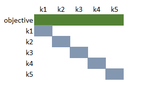Structure of the combined model (after reordering)

LP solvers do not really try to exploit this structure and just look at it as a big, sparse matrix.

This looks like a somewhat special case: many, independent, very small MIP models. However, I have been involved in projects dealing with multi-criteria design problems that had similar characteristics.

Conclusions:

• The end result: even for 1000 random scenarios, we can find in each case two teams that have exactly the same average ELO rating.
• Solving many different independent scenarios may require some attention to achieve best performance. 

References

1. Selecting Chess Players, https://yetanothermathprogrammingconsultant.blogspot.com/2018/11/selecting-chess-players.html