Monday, November 30, 2015

Linearization by enumeration for a small reliability problem

In http://yetanothermathprogrammingconsultant.blogspot.com/2015/11/global-optimality.html a small MINLP model is shown that does not solve that easily. Here is it again:

image

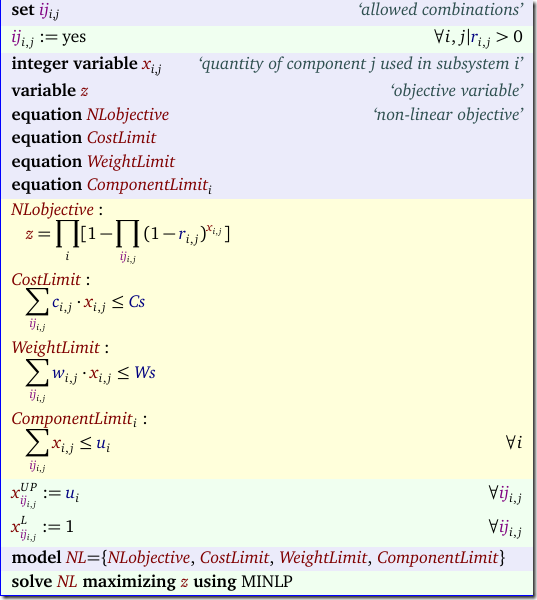
The model and the data comes from: A Hybrid Parallel Genetic Algorithm for Reliability Optimization. The model is called RRAP for Reliability-Redundancy Allocation Problem. We allow for a mix of redundant components to maximize total system reliability with some weight and cost constraints. For small problems we can use a simple mechanism to linearize the objective: just enumerate the possible configurations for a subsystem i. In this case we have only 4 different components in a subsystem and we can have at most u(i)=6 components in total in each subsystem. That means we can enumerate all possible combinations:

image

In total: 209 combinations for the most complex sub-systems. Using this enumeration scheme we can use a binary variable to indicate whether we select a certain combination. With this we can form a linear model:

image

We can drop the ComponentLimit constraint as this is now part of the enumeration process. Notice that our model is simpler than the one stated in the paper which looks somewhat strange here and there, as if they got lost a little bit in the math. E.g. for the cost and weight limits the paper proposes:

image

I like my version much better.

The objective coefficients coeff(i,k) are calculated as:

image

Note: the subset ik(i,k) indicates that not all possible combinations (i,k) are allowed: some subsystems i have fewer possible configurations k. Also note that we are maximizing log(z) instead of z. But as this is a monotonic transformation, this will give us the same optimal solution.

As the problem is small, the final MIP is also not too big. It has a simple structure and good MIP solvers solve this very fast. This is a fairly standard way of dealing with these kind of problems, so it should be in our toolbox.

Saturday, November 28, 2015

BLEIC

I never came across this acronym: BLEIC: Boundary and Linear Equality/Inequality Constrained Optimization. I usually use “linearly constrained NLP”.

I saw this in: http://www.angoss.com/predictive-analytics-software/software/insightoptimizer/.  Lots of PR language on this page and not much technical details. Seems like modeling by clicking on buttons.

Friday, November 27, 2015

Global optimality

Not sure if this is a bug or this just comes with the territory (i.e. numerics). When I solve this nasty MINLP with Baron using an allowed gap optcr=0 I get:

Solution      = 0.922492168619502  found at node 6
Best possible = 0.92249216962
Absolute gap  = 1.00049823981152E-9  optca = 1E-9
Relative gap  = 0.00000  optcr = 1E-9

This is actually very good performance. However there is better solution (we are maximizing). If I plug this solution into the model I see:

Solution      = 0.954564813873509  best solution found during preprocessing
Best possible = 0.954564813874
Absolute gap  = 4.91051643791707E-13  optca = 1E-9
Relative gap  = 0.00000  optcr = 1E-9

This is somewhat better (about 3% improvement). This looks like a little bit more than expected.

The model is related to some reliability problem:

image

Tuesday, November 24, 2015

This can be done much better

Counter example of how to present a model in a paper:

image

I suspect the reason why I often see names like x1,x2,… being used, is that some textbooks present models that way. In this respect computer science and programming has made more progress: no paper or book would use such variable names anymore.

Sunday, November 15, 2015

Configuration files

Often I use INI files (https://en.wikipedia.org/wiki/INI_file) for configuration settings of programs I develop. For programs that need more complicated data structures one could use XML or JSON. Here is a good alternative for JSON: http://hjson.org/.

image

There is some source code to store the comments along with the real data when reading an HJSON file. That is useful to preserve comments when updating the configuration file by a program.

I have also seen a suggestion to use SQLite to store configuration settings.

Thursday, November 12, 2015

Example of supplier selection with discounts

I am working on a supplier selection model, so it is useful to see how my formulation compares to what others have come up with. The next paper is not really identical to my situation but it is useful to look at it anyway. (In my case I have more strange discount and incentive rules – it is amazing what sales people can come up with to make you buy their product – and we also want to look at procurement and administrative cost and at the impact of limiting the number of suppliers).

image

This model involves selecting carriers for shipping. The notation and data used is as follows:

image

We have i shipping companies to select from, and j transportation links we need to send goods along. Not every shipper handles all lanes. There is a simple discount schedule for each shipper: when we ship more than certain thresholds we get a discount on all shipments using this carrier. The model the paper proposes is:

image

This is a small, compact and simple model, but nevertheless there are many points we can make about this model:

image

  1. The objective is missing an = sign after the ω. I.e. ω is not a weight on the first term in the objective but rather an objective variable. OK, no big deal, just a typo.
  2. The second issue is more of a real modeling problem. I see this often: expressions are repeated in the model. In general this is bad idea. It is better to add variables and equations to the model so that we don’t have to repeat whole expressions. This can save a lot of non-zero elements in the model and make the model sparser. Even though we add variables and equations to the model, usually this is a worthwhile reformulation.
  3. Big M values in the model are always a problem. Especially as stated like this: one value M for all cases. We need to choose tight values for these. I see many models with large big M values causing problems for MIP solvers. In the first case we can use an alternative formulation which is even simpler:
    image
    Note that we replaced the sum by a new variable y.
  4. This one can also be reformulated by introducing a parameter γi,k (gamma) indicating the upper bound of the discount interval. Of course we have γi,ki,k+1. The inequality can now become:
    image 
    It is interesting to verify why the original version worked. It just looks at the lower bound of each interval. It is relying on discounts to increase when we move to a higher discount interval. The objective will then select the best interval. In my reformulated version we don’t rely on the objective but rather force the z to indicate the interval. In my formulation for a given z we will never be outside the corresponding interval. See also: http://yetanothermathprogrammingconsultant.blogspot.com/2015/10/discontinuous-piecewise-linear.html.
  5. This equation fixes a lot of variables to zero. Besides writing this as a bound instead of an equation, we can actually make sure we never generate those inadmissible assignments. Solvers have very good presolvers that will remove these kind of equations, but in general I prefer to do this myself. I am always worried if the presolver is reducing my model by a large amount. Of course this is not always a modeling problem: if the model has a large triangular structure, we may see that the presolver takes a big bite out the model.
  6. This is an interesting way to force some risk adjustment: we don’t want a single shipper to be the only and dominant shipper over a given lane. Therefore it can not handle more than q*100% of the shipments over a link. In practice one would want to see what the trade-offs are between cost and this risk measure.

The authors claim the MIP formulation does not solve fast enough for large instances so they developed a heuristic. I was able with some reformulations and some tinkering to solve the large instances within a few minutes to a 1% gap. Current MIP solvers are very good in finding good solutions very quickly. MIP solvers also have the unique capability to establish the quality of a solution (the gap). Note that this gap is often somewhat conservative. When we stop on a 1% gap, most likely we are much closer to the optimal solution than this 1% (but not guaranteed).

There are sometimes very good reasons to use heuristics. However I believe in quite a few cases developers prematurely dismiss MIP models, sometimes based on poorly formulated models.