Monday, June 29, 2009

Cbc/glpk

There is an option in Coin-or’s CBC to include the modeling language from glpk. This is a reasonable subset of AMPL. I tried to compile this quickly but it took me longer than expected, mainly because the CBC sources are not updated for the latest glpk versions which have a different API.

Some observations:

  • The configure script is very time consuming: it is checking for the C++ compiler again and again (for each subsystem).
  • It was a little bit trial and error to convince the system to include glpk. I looked briefly (may be too briefly) for documentation.
  • The glpk system is considered just another input format. The sources of the glpk integration are actually embedded in the source file for reading MPS files. This means that the output (solution) is not brought back to glpk so no report writing in glpk is available.
  • I suspect the solution file has no names but only numbers (I tried different things without avail but may be there is a way). How to map names to numbers? Don’t know.
  • May be cbc should be called from glpk instead of the other way around. That would deal with a number of the issues mentioned here.
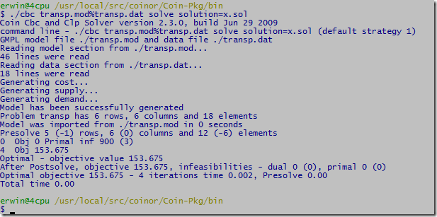
  • To process the file use xxx.mod%xxx.dat or xxx.mod% on the command line (see screen dump below).

cbcglpk

Friday, June 26, 2009

Duplicate rows

I saw a model with:

Const_A5 {i in D, j in S : j!=1 }: (- 1.1) * TA[j] + TA[j-1] + 0.1 * AC[j] - 4 * W['A',j] + 0.1 * OT[j] + 2 = 0 ;

this really generates duplicate constraints: the above constraint is repeated for each i in D. A simpler example would be:

supply{k in K,i in I}: sum{j in J} x[i,j]  <=  a[i] ;

or in GAMS: 

supply(k,i) ..   sum(j, x(i,j))  =L=  a(i) ;

Both AMPL, GLPK and GAMS just generate these duplicates without a problem.

I cannot think of a case where such construct is very useful in practice, so modeling languages should probably flag this as an error (or at least a warning).

Some really good presolvers can get rid of this, but this seems an opportunity where a modeling system can give useful feedback to an innocent user.

PS. To debug these cases GAMS has an equation and variable listing controlled by option LIMROW and LIMCOL. Ampl has an `expand’ command to show what is generated. With Glpsol it is often useful to generate a Cplex LP file to see what is generated.

Thursday, June 25, 2009

gsl vs lapack performance

I had some doubts about the LU routines in the gsl library (GNU Scientific Library). See http://yetanothermathprogrammingconsultant.blogspot.com/2009/06/gsl-gnu-scientific-library.html. Here I try a quick experiment by inverting a square nxn matrix. As test matrix I used the Pei matrix (http://portal.acm.org/citation.cfm?id=368975). Here are the results:

library gsl lapack
routine gsl_linalg_LU_decomp +
gsl_linalg_LU_invert
dgesv
compiler cygwin gcc Lahey lf95
n=100 0.047 seconds 0.024 seconds
n=1000 6.735 seconds 2.017 seconds
n=2000 1:01 minutes 17.257 seconds

Indeed it looks that gsl is not quite competitive with lapack for this operation (although much better than figures I displayed earlier – these were wrong). I suspect this is due to how the gsl routines access many of the matrix elements: through an inlined function with the complicated expression m->data[i * m->tda + j]. I think the fast C way of doing this is to use pointers and pointer arithmetic. Another issue is cache misses. One should run through the matrix so that memory accesses as as much localized as possible.

PS. Of course it is noted that in most cases you do not want to invert a matrix, but rather solve for a given rhs.

PS2. Sorry: previous lapack timings were wrong (the input matrix was by accident zero for off-diagonal elements, that makes the inversion very simple!).

Tuesday, June 23, 2009

Subversion book

http://svnbook.red-bean.com/

This version control tool (svn server + tortoise client) can be useful for larger modeling projects.

Notes:

  • To bypass firewalls/routers use http protocol via Apache
  • Diff of Excel files seems to work with tortoise (cells that are different are shown in red)

Xpress forum moved

New location is http://discuss.fico.com/blaze/board?board.id=xpressdiscuss.

Visual Studio C# debug problem

This is not very helpful: I am hitting an Debug.Assert in some C# code (I am running in debug mode). When I want to look any local variable in the method I see:

cannot evaluate expression because the code of the current method is optimized

It has to do with the Assert. After rewriting as an if statement so I can place a breakpoint I can inspect all variables.

Others have reported the same: http://connect.microsoft.com/VisualStudio/feedback/ViewFeedback.aspx?FeedbackID=278033. The answer seems somewhat a cop-out: Closed (Not Reproducible).

I have seen similar issues with Delphi. This is always annoying: when you are debugging you want to focus on the problem at hand, and such debugger bugs suddenly make you pay attention to other things.

Sunday, June 21, 2009

Simplex method description

A comment led me to visit https://hudson.jboss.org/hudson/job/drools/lastSuccessfulBuild/artifact/trunk/target/docs/drools-solver/html_single/index.html. Section 1.3.1.3 has an interesting statement about the Simplex method:

Simplex turns all constraints and data into a big equation, which it transmutes into a mathematical function without local optima. It then finds an optimal solution to the planning problem by finding an optima of that mathematical function.

If the word Simplex was missing I would not recognize this is about the Simplex method. One big equation? (No word about not being suited to handle discrete variables).

The branch&bound section is also interesting. No mention about the unique feature that it provides bounds and hence an indication of the quality of the solution.

Friday, June 19, 2009

Standard Formulations

Sometimes it helps if a modeler has a toolbox with a number of standard formulations available for recurring problems so attacking new situations becomes just an incremental effort. An example is discussed here: http://code.msdn.microsoft.com/solverfoundation/Thread/View.aspx?ThreadId=1888. The original poster got a little bit lost by reinventing a formulation for a standard production scheduling problem with a twist. Reusing the standard inventory balance formulation helped simplify the model after which adding the extra complication of allowing next day delivery was easy.

Thursday, June 18, 2009

Coin-or CBC install

I hoped that this would work without problem on a freshly installed, vanilla Cygwin environment:

$ svn checkout https://projects.coin-or.org/svn/Cbc/releases/2.3.0 Coin-Pkg
$ cd Coin-Pkg/
$ ./configure
$ make
$ make install

The last messages I see are:

Making install in Clp
make[1]: Entering directory `/usr/local/src/coinor/Coin-Pkg/Clp'
Making install in src
make[2]: Entering directory `/usr/local/src/coinor/Coin-Pkg/Clp/src'
.deps/CbcOrClpParam.Po:1: *** multiple target patterns.  Stop.
make[2]: Leaving directory `/usr/local/src/coinor/Coin-Pkg/Clp/src'
make[1]: *** [install-recursive] Error 1
make[1]: Leaving directory `/usr/local/src/coinor/Coin-Pkg/Clp'
make: *** [install-recursive] Error 1

This is in the ‘make install’ step. I don’t know what a .Po file is, nor why it is in a hidden directory .deps.

Wednesday, June 17, 2009

Defined Variables

For some NLP models defined variables can help to reduce the size of the optimization model while maintaining readability. Defined variables are variables that will be removed by the modeling system by substitution. Sometimes introduction of defined variables in the model requires a little bit of thought. In this example we consider a maximum likelihood estimation problem of a GARCH(p,q) process. GARCH time series are often used in financial applications.

The GARCH(p,q) model can be described as:
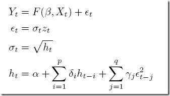
garch1 where εt follows a process described by the last three equations and zt has a Gaussian distribution. We assume the simplest functional form for F:

garch2 i.e. a constant value. The parameters to estimate are θ=(μ,α,δij). The optimization problem for finding these can be written as:

garch3where we maximize the log likelihood function subject to some stationarity condition. We can simplify the objective to:

garch4

In this document I describe a GAMS implementation. We use extra variables for εt and ht. The basic model looks like:

variables
   L       
'log likelihood (constants taken out)'
   h(t)    
'sigma(t)=sqrt(h(t))'
   e(t)    
'residuals'
   alpha_0 
'GARCH parameter (constant)'
   alpha(q)
'GARCH parameters (q)'
   beta(p) 
'GARCH parameters (p)'
   constant
'information structure: y = constant + e'
;


equations
   loglike     
'transformed log likelihood function'
   def_h(t)    
'h(t) structure'
   stat_garch  
'stationarity condition (GARCH model)'
   series(t)   
'defines the time series'
;

loglike..       
L =e= sum(lag(t), log(h(t)) + sqr(e(t))/h(t) );
def_h(lag(t))..  h(t) =e= alpha_0 +
sum(q, alpha(q)*sqr(e(t-ord(q))))
                                 +
sum(p, beta(p)*h(t-ord(p))) ;
stat_garch..    
sum(q,alpha(q)) + sum(p,beta(p)) =l= 1;
series(lag(t)).. y(t) =e= constant + e(t);


model garch /loglike, def_h, stat_garch, series/;
solve garch using nlp minimizing L;

Here lag is a subset so we don’t go beyond the border when evaluating lagged variables ht-i and εt-j. Note that we have many more variables in this model than original stated. Especially ht and εt contribute. The model statistics are:

MODEL STATISTICS

BLOCKS OF EQUATIONS           4     SINGLE EQUATIONS        2,084
BLOCKS OF VARIABLES           7     SINGLE VARIABLES        2,089
NON ZERO ELEMENTS        10,413     NON LINEAR N-Z          6,246
DERIVATIVE POOL           2,089     CONSTANT POOL              16
CODE LENGTH              40,602

The results for the GARCH(1,1) case are:

----    439 VARIABLE L.L                   =      329.732  log likelihood (constants taken out)
            VARIABLE alpha_0.L             =        0.019  GARCH parameter (constant)

----    439 VARIABLE alpha.L  GARCH parameters (q)

q1 0.042

----    439 VARIABLE beta.L  GARCH parameters (p)

p1 0.919

Can we reproduce with AMPL using defined variables? Not very difficult. The real problem is how to deal with ht and εt for t ≤ max(p,q)+1. The GAMS model actually lets them float. The εt‘s are small so we can just fix them: it would not make much difference in the solution. Actually I believe in the GAMS model we should have used:

series(t1(t)).. y(t) =e= constant + e(t);

The initial ht‘s are more important. Lets try to mimic the GAMS implementation here. We do that with an additional variable h0. The complete AMPL model looks like:

set T ordered;

param s{T};

set T1 ordered := T diff {first(T)};

param y{t in T1} := 100*log(s[t]/s[prev(t,T)]);

param p = 1;
param q = 1;
param mpq = max(p,q);

# create a set where we drop the first mpq entries from T1
set Lag ordered := {i in T1: ord(i,T1) > mpq};

var constant;
var alpha_0 >= 0.0001, <= 100, := .1;
var alpha{i in 1..q} >= 0, <= 100, := .1;
var beta{j in 1..p} >= 0, <= 100, := .1;

var e{t in T1} = y[t] - constant;
set T0 := T1 diff Lag;
var h0{t in T0} >= 0.0001;
var h{t in T1} =
     if (t in Lag) then (alpha_0 + sum{i in 1..q} alpha[i]*e[prev(t,T,i)]^2
                     + sum{j in 1..p} beta[j]*h[prev(t,T,j)])
               else h0[t];

minimize L: sum{t in Lag} (log(h[t]) + e[t]^2/h[t]);

stat_garch: sum{i in 1..q} alpha[i] + sum{j in 1..p} beta[j] <= 1;

This generates a very small model:

Substitution eliminates 2084 variables.
Adjusted problem:
5 variables, all nonlinear
1 constraint, all linear; 2 nonzeros
1 nonlinear objective; 5 nonzeros.

MINOS 5.5: optimal solution found.
30 iterations, objective 329.731725
Nonlin evals: obj = 85, grad = 84.
ampl: display L,alpha_0,alpha,beta;
L = 329.732
alpha_0 = 0.0194425

:     alpha       beta      :=
1   0.0415491   0.919192
;

This indeed is much smaller than the GAMS model. The exercise was also useful as it revealed some soft spots in the GAMS formulation. I probably need to rethink how we deal with initial ht‘s in the GAMS model: the results are sensitive to how this is handled.
Saturday, June 13, 2009

Generated models

When programs generate models in MathProg/AMPL they tend to have a different structure. In this case a scalar model was generated with some very long lines. The user reports some very large memory usage:

Model has been successfully generated
glp_simplex: original LP has 93 rows, 5256 columns, 84143 non-zeros
glp_simplex: presolved LP has 82 rows, 5256 columns, 77163 non-zeros
Scaling...
A: min|aij| =  1.000e+00  max|aij| =  1.600e+02  ratio =  1.600e+02
GM: min|aij| =  4.952e-01  max|aij| =  2.019e+00  ratio =  4.077e+00
EQ: min|aij| =  2.471e-01  max|aij| =  1.000e+00  ratio =  4.048e+00
Crashing...
Size of triangular part = 82
      0: obj =   0.000000000e+00  infeas =  5.657e+00 (0)
*    50: obj =   1.410800000e+00  infeas =  0.000e+00 (0)
*    80: obj =  -7.209526707e-32  infeas =  2.776e-17 (0)
OPTIMAL SOLUTION FOUND
Time used:   0.1 secs
Memory used: 2008.7 Mb (2106232859 bytes)

(With some versions it may even stop with a stack overflow). Indeed this is due to the modeling language part and not the solver per se. When we run:

$ glpsol --math big.mod --wcpxlp big.lp
$ glpsol --cpxlp big.lp

the second invocation will just use a fraction of the memory. Clearly glpk has troubles with very long scalar expressions.

Actually AMPL is not doing much better:

big.mod, line 7005 (offset 158374):
        HES03 is not defined

Looks like we hit a max line length limit, and a variable name is truncated leading to this error. A better message would be “line is too long”. Even better is not to have artificial limits on input lines.

I remember reports about similar issues with early versions of the GCC compiler: it had problems with machine generated C code where expressions were spanning several pages. This was very different from how a normal programmer would write code.

GSL: GNU Scientific Library

I was looking into the GSL for a project. I am puzzled about the design of the LU solver. To solve a system of linear equations Ax=b, one would call gsl_linalg_LU_decomp followed by gsl_linalg_LU_solve. The strange thing is: non of these functions has a return code for “sorry: the matrix was singular”. When passing a singular matrix both routines will return GSL_SUCCESS.

I thought it would be a good idea to give the GSL people some feedback on this: http://lists.gnu.org/archive/html/bug-gsl/2009-06/msg00005.html.

Looking at the linear algebra code, I have to say the implementation looks rather unsophisticated compared to say LINPACK or LAPACK.

Update: the GSL people answered here. Better than nothing, but not optimal. You really want this flag in the decomposition as it is detected there, and because it makes it easier to write:

call decomp(A);
if not singular then
   for i := 1 to NumRHS do
      call solve(rhs[i]);

Never thought I would say this, but it looks like LINPACK/LAPACK is more user-friendly than GSL in this respect.

Thursday, June 11, 2009

AMPL error message

This is not a very informative error message:

sw: ampl
ampl: var b, binary;
var h;

maximize obj: b;

e: b=0 <==> h>=0;

option solver cplex;
solve;
Error executing "solve" command:

    unexpected type 0x920c in lsimplify()
sw:

I believe error messages are the “user interface” when it really matters: when the user is confused. The value of good error messages is often underestimated. Of course we can assume the developer never thought this message would be issued.

I tried the implication based on information in http://www.ampl.com/INFORMS06.pdf. I assume this has to be written as

e: b=0 ==> h>=0 else h<=-0.0001;

or

e: b=0 ==> h>=0 else h<=0;

if the ambiguity about h=0 is no problem.

Wednesday, June 10, 2009

.NET profiler

I wanted to have a look at where I spend my time in a C# application. This profiler from http://www.eqatec.com/tools/profiler helped me to find some issues in my code. The user interface is very intuitive.


Saturday, June 6, 2009

Large easy LP’s: are modeling systems fast enough?

> I am planning to solve some fairly large network-like LP problems. I assume it is not a good idea to use a modeling language: it will slow things down too much.

Well, it depends. Of course specialized software will be much faster than a modeling language with an LP solver. But you should not underestimate what can be solved these days. Here is an (artificial) example of a pure network model. I took the “trnsport” model from the GAMS model library and scaled it up by duplicating it 200,000 times. That will give us a (quite dense) transportation problem with 1 million rows and 1.2 million columns.

Sets
     k  
duplicate        / instance1*instance200000 /
     i  
canning plants   / seattle, san-diego /
     j  
markets          / new-york, chicago, topeka / ;

Parameters

     a(i) 
capacity of plant i in cases
      
/    seattle     350
           
san-diego   600  /

     b(j) 
demand at market j in cases
      
/    new-york    325
           
chicago     300
           
topeka      275  / ;

Table d(i,j)  distance in thousands of miles
                 
new-york       chicago      topeka
   
seattle          2.5           1.7          1.8
   
san-diego        2.5           1.8          1.4  ;

Scalar f  freight in dollars per case per thousand miles  /90/ ;

Parameter c(i,j)  transport cost in thousands of dollars per case ;

          c(i,j) = f * d(i,j) / 1000 ;

Variables
     x(k,i,j) 
shipment quantities in cases
     z        
total transportation costs in thousands of dollars ;

Positive Variable x ;

Equations
     cost         
define objective function
     supply(k,i)  
observe supply limit at plant i
     demand(k,j)  
satisfy demand at market j ;

cost ..        z  =e= 
sum((k,i,j), c(i,j)*x(k,i,j)) ;

supply(k,i) ..  
sum(j, x(k,i,j))  =l=  a(i) ;

demand(k,j) ..  
sum(i, x(k,i,j))  =g=  b(j) ;

Model transport /all/ ;

option iterlim=1000000;
Solve transport using lp minimizing z ;

Running this with a good LP solver with all default settings gives the following results:

Solver Cplex Gurobi
GAMS generation time (seconds) 10.4 10.4
Solver time (seconds) 78.6 48.4
total turnaround time (mm:ss) 1:38 1:20

We see that the LP solver still uses most of the total time.

Now lets see what happens if we fine-tune a bit. Let’s turn off some of the massive listing output GAMS is generating, and let it dump the solution in a binary GDX data-file. Also let’s see what happens if we use Cplex’s network and barrier solvers. We can do this with:

Model transport /all/ ;

option limrow=0;
option limcol=0;
option iterlim=1000000;
transport.optfile=1;
transport.solprint=0;
Solve transport using lp minimizing z ;

execute_unload 'sol.gdx',z,x;

$onecho > cplex.opt
lpmethod 3
$offecho

The results are:

Solver Cplex
Network
Cplex
Barrier
Id.
No Crossover
GAMS generation time (seconds) 6.4 6.4 6.4
Solver time (seconds) 22.2 19.1 13.3
total turnaround time (mm:ss) 0:31 0:28 0:25

With the fastest solver settings we see that the solver uses about half of the total turn-around time.

For this model GAMS is holding up quite nicely. Conclusion: easy, large LP’s do not immediately imply that a modeling system should not be used because of performance reasons. I conjecture that the reason for this is as follows. If all is OK, GAMS should be able to generate models in roughly linear time w.r.t. the number of non-zeroes of the model. Solvers have worse run-time complexity, so they will start to get slower in relative terms when the problem is getting really big. For difficult LP’s and for MIP models especially, the solver will use in general (much) more time than GAMS. An exception is when LP restarts are used: sometimes LP solvers can very efficiently use an advanced basis to find the optimal solution of a related model. GAMS is not very intelligent in generating such restart models (it will generate each model essentially from scratch). Some other modeling systems such as AIMMS have special facilities to do this faster. For surprisingly many models the GAMS approach actually works just fine.

Of course there may be many other issues that can influence your decision: software acquisition cost, model development cost, model maintenance issues, your current skills and familiarity with modeling software, preferences (“I like to program in C”) etc.

Thursday, June 4, 2009

NEOS: SCIP indicator constraints with AMPL

The question came up whether Cplex is the only solver that supports indicator constraints. It looks like SCIP supports these also: http://scip.zib.de/doc/html/cons__indicator_8c.html. I tried this with the the NEOS setup at http://www-neos.mcs.anl.gov/neos/solvers/milp:scip/AMPL.html but that seems to have a rather unsophisticated AMPL link to put it mildly. As only minimization is allowed it looks like it is going through an MPS file. As a result the AMPL indicator constraints are also not available. The error message I receive when I submit a test model with an implication is a little bit off:

ERROR: Runtime error encountered


2 variables, all nonlinear
0 algebraic constraints
1 logical constraint
1 linear objective; 2 nonzeros.
Problem has 2 nonlinear variables.  No MPS file written.


Please correct and resubmit.

The model is really linear. I suspect AMPL uses nonlinear functions as a mechanism to communicate the logical constraints with the solver.

I like the concept of indicator constraints and how they are implemented in AMPL (http://www.ampl.com/INFORMS06.pdf). I would certainly hope other solvers would also move into this direction. Given the increasing attention for Constraint Programming, it makes sense to expect that these features get more traction. I also tried to check the GAMS documentation on GAMS/SCIP to see what GAMS has to offer here. Unfortunately the documentation for GAMS/SCIP is largely nonexistent: http://www.gams.com/dd/docs/solvers/coin.pdf.

Tuesday, June 2, 2009

Using awk from GAMS to split set elements

I have a set with

ARG_BT_EX
ARG_BT_IM
ARG_BT_NT
ARG_BT_QC

Now I want to extract from this three sets: Country (ARG), Commodity (BT) and Other (EX,..).

This can be done easily with AWK:

$onecho > baseset.inc
ARG_BT_EX
ARG_BT_IM
ARG_BT_NT
ARG_BT_QC
ARG_BT_QP
$offecho

$onecho > gen.awk
BEGIN{
  FS="_"
}
{
  print $0 "." $1 "." $2 "." $3
}
$offecho

$call awk.exe -f gen.awk baseset.inc > extset.inc

set i(*) /
$include baseset.inc
/;

set imap(i,*,*,*) /
$include extset.inc
/;

alias (*,s1,s2,s3);

set country(*);
set commodity(*);
set other(*);

loop(imap(i,s1,s2,s3),
  country(s1) = yes;
  commodity(s2) = yes;
  other(s3) = yes;
);

execute_unload "sets.gdx",imap,i,country,commodity,other;

The AWK script will generate the mapping set imap:

ARG_BT_EX.ARG.BT.EX
ARG_BT_IM.ARG.BT.IM
ARG_BT_NT.ARG.BT.NT
ARG_BT_QC.ARG.BT.QC
ARG_BT_QP.ARG.BT.QP

while the rest of the GAMS code will extract the individual sets from this compound set.

AWK is included in the Windows versions of GAMS.

GAMS: Piecewise linear functions with SOS2 variables

Sometimes we need to represent a piecewise linear function, like:

sos2-1

This can be modeled with the following:

sos2-2

Equation (1) is called the “reference row”, equation (2) the “function row” and equation (3) the “convexity row”. Many MIP solvers have so-called SOS2 facilities: special ordered sets of type 2. The lambda variables form a SOS2 set, so this makes using this very simple (it is possibly to simulate this with extra binary variables). In GAMS this looks like:

variables y,x;
sos2 variables lambda(k);

equations refrow, funrow, convexity;

refrow.. x =e= sum(k, lambda(k)*xbar(k));
funrow.. y =e= sum(k, lambda(k)*ybar(k));
convexity.. sum(k, lambda(k)) =e= 1;

Notes:

  • It is important to keep the “set-index” last. See the fragment of a model I am working at now:

defq(i,t).. q(i,t) =e= sum(ic(i,c), lambda(i,t,c)*xpoints(c));

defcost(i,t)..  cost(i,t) =e= sum(ic(i,c), lambda(i,t,c)*ypoints(i,c));

convex(i,t)..  sum(ic(i,c),lambda(i,t,c)) =e= 1;

Here we need to keep c last in variable lambda. This makes sure we have i × t sets with c members. In this case c is dependent on i through the set ic(i,c).

  • AMPL has special language constructs to make this even easier.
  • MS Solver Foundation also has added SOS2 support.
  • GAMS has no facility to specify the reference weights (they are usually automatically generated to be 1,2,…).  Of course in many cases I can not make a good use of reference weights anyway, as I would not know any better values.