Adaptive Strawberry Algorithm?

In (1) a so-called Adaptive Plant Propagation or Adaptive Strawberry Algorithm is applied to a standard Economic Load Dispatch problem.

I had never heard of adaptive strawberries or about this dispatch problem being difficult enough to warrant a heuristic approach.

Abstract

Optimization problems in design engineering are complex by nature, often because of the involvement of critical objective functions accompanied by a number of rigid constraints associated with the products involved. One such problem is Economic Load Dispatch (ED) problem which focuses on the optimization of the fuel cost while satisfying some system constraints. Classical optimization algorithms are not sufficient and also inefficient for the ED problem involving highly nonlinear, and non-convex functions both in the objective and in the constraints. This led to the development of metaheuristic optimization approaches which can solve the ED problem almost efficiently. This paper presents a novel robust plant intelligence based Adaptive Plant Propagation Algorithm (APPA) which is used to solve the classical ED problem. The application of the proposed method to the 3-generator and 6-generator systems shows the efficiency and robustness of the proposed algorithm. A comparative study with another state-of-the-art algorithm (APSO) demonstrates the quality of the solution achieved by the proposed method along with the convergence characteristics of the proposed approach.

Problem

The economic dispatch problem used in this paper can be stated as a simple convex QP (Quadratic Programming) problem:

\[\bbox[lightcyan,10px,border:3px solid darkblue]{
\begin{align}\min\>&z = \sum_i (a_i + b_i x_i + c_i x_i^2)\\
& \sum_i x_i = D\\
& \ell_i \le x_i \le u_i\end{align} } \]

Basically with have \(n\) generators that have a quadratic cost function w.r.t. to their output \(x_i\). The constraints deal with meeting demand and operating limits.

Nitpick: the paper mentions: \(\ell_i < x_i < u_i\) which is mathematically not really ok.

Opposed to what the abstract is saying this is not a non-convex problem, and standard QP algorithms will be able to solve this problem without any problem. There really is no good reason for using a heuristic for this problem.

Example 1

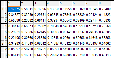
The first example is a tiny problem with three generators.

Note that the columns in table 1 are mislabeled. The first column represents \(c_i\) while the last column is \(a_i\).

The solution is reported as:

The solution calculated by hand seems correct (I guess the author was lucky here that no operating limits were binding). The heuristic gives a solution that is slightly better (lower cost) but that is because this solution is slightly infeasible: we don’t quite match the demand of 800 MW. 

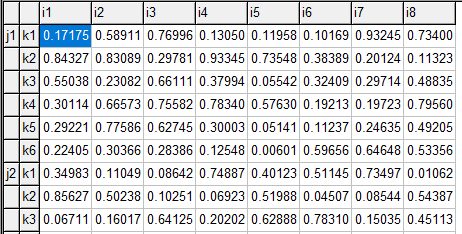
Example 2

This is another tiny problem with six generators.

The demand is 410 MW. The author shows two solutions:

These solutions are both wrong. The reported objective values (Cost per hour) should be an indication something is not right. The reason is that the author is confused about the (mislabeling of the) coefficients \(a_i\), \(b_i\), \(c_i\) in table III. The large coefficients \(C_i\) deal with the fixed cost while the small coefficients \(A_i\) are for the quadratic terms.

The correct solution is:

A QP solver can solve this model to (proven) optimality in less than a second (Cplex takes 0.09 seconds).

Unit Commitment Problem

A more interesting problem is where we can turn generating units on and off. This is called the unit-commitment problem. Often exotic things like ramp-up and ramp-down limits, and other operational constraints, are added. These problems can actually become very difficult to solve, and heuristics pay traditionally an important role here. Having said that, there is somewhat of an increased interest to solve these models with MIP technology (after piecewise linear representation of the quadratic costs) due to substantial advances in state-of-the-art solvers. I have not seen many efforts to use MIQP algorithms here: often these linearized versions work quite well.

Conclusion

Writing a solid paper is not that easy.

References

1. Sayan Nag, Adaptive Plant Propagation Algorithm for Solving Economic Load Dispatch Problem, 2017 [link]

Quantiles

Calculating quantiles is a standard way to summarize data. In the example below we have some small random data p(i,j,k) where we want to calculate quantiles at the 0, 25, 50, 75, and 100% level for each (i,j):

----      9 PARAMETER p                 k1          k2          k3          k4          k5          k6          k7          k8 i1.j1      18.003      84.483      55.487      30.813      29.929      23.181      35.633      85.771 i1.j2       7.644      50.521      99.814      58.295      99.122      76.463      13.939      64.332 i1.j3      16.792      25.758      67.224      44.100      36.610      35.793      14.018      15.860 i2.j1      59.322      83.258      23.851      66.908      77.810      31.062      11.939      50.736 i2.j2      16.857      87.374      27.246      29.296      59.802      72.549      63.197      46.916 i2.j3      41.917      12.652      32.107       5.609      34.516      19.028      64.927      56.514 ----    143 PARAMETER quantiles                 0%         25%         50%         75%        100% i1.j1      18.003      28.242      33.223      62.736      85.771 i1.j2       7.644      41.375      61.313      82.128      99.814 i1.j3      14.018      16.559      30.775      38.483      67.224 i2.j1      11.939      29.259      55.029      69.633      83.258 i2.j2      16.857      28.783      53.359      65.535      87.374 i2.j3       5.609      17.434      33.312      45.566      64.927

In GAMS this is not so easy. Here is one way:

set i /i1*i2/     j /j1*j3/     k /k1*k8/     q /'0%', '25%', '50%', '75%', '100%'/ ; parameter p(i,j,k); p(i,j,k) = uniform(1,100); display p; parameter    v(k) 'vector to be sorted'    r(k) 'sorting rank'    perc0(q) /'0%' EPS, '25%' 25, '50%' 50, '75%' 75, '100%' 100 /    perc(q) 'percentiles'    quantiles(i,j,q) ; $libinclude rank loop((i,j),   v(k) = p(i,j,k);   perc(q) = perc0(q); $ libinclude rank v k r perc   quantiles(i,j,q) = perc(q); ); display quantiles;

We use here the rank utility by Tom Rutherford. A disadvantage is that it is designed to work on vectors. That means we need to loop to extract a k-vector. Under the hood a GDX file is written for each vector, a program called gdxrank is called, and another GDX file is written with the ranks of each vector element. For very large data sets this turns out to be very slow.

Note that in the data statement for perc0 we use EPS instead of 0. This on purpose: EPS will survive the trip to gdxrank, while a pure zero is not stored and not transmitted. If we would have used 0 instead of EPS we would have seen:

----    142 PARAMETER quantiles                25%         50%         75%        100% i1.j1      28.242      33.223      62.736      85.771 i1.j2      41.375      61.313      82.128      99.814 i1.j3      16.559      30.775      38.483      67.224 i2.j1      29.259      55.029      69.633      83.258 i2.j2      28.783      53.359      65.535      87.374 i2.j3      17.434      33.312      45.566      64.927

How would this look in R?

R has the quantile function to calculate percentiles of a vector. We can use the by function to apply this on a slice of the data. This can look like:

> df     i  j  k     value 1  i1 j1 k1 18.002966 2  i1 j1 k2 84.483404 3  i1 j1 k3 55.487160 4  i1 j1 k4 30.812652 5  i1 j1 k5 29.929000 6  i1 j1 k6 23.181234 7  i1 j1 k7 35.633220 8  i1 j1 k8 85.770764 9  i1 j2 k1  7.644259 10 i1 j2 k2 50.520856 11 i1 j2 k3 99.813645 12 i1 j2 k4 58.294604 13 i1 j2 k5 99.122171 14 i1 j2 k6 76.462796 15 i1 j2 k7 13.938556 16 i1 j2 k8 64.332157 17 i1 j3 k1 16.792269 18 i1 j3 k2 25.757973 19 i1 j3 k3 67.223932 20 i1 j3 k4 44.100282 21 i1 j3 k5 36.610326 22 i1 j3 k6 35.792695 23 i1 j3 k7 14.017667 24 i1 j3 k8 15.860077 25 i2 j1 k1 59.322251 26 i2 j1 k2 83.258388 27 i2 j1 k3 23.850758 28 i2 j1 k4 66.907712 29 i2 j1 k5 77.809903 30 i2 j1 k6 31.062189 31 i2 j1 k7 11.938737 32 i2 j1 k8 50.736102 33 i2 j2 k1 16.857103 34 i2 j2 k2 87.373769 35 i2 j2 k3 27.246340 36 i2 j2 k4 29.295618 37 i2 j2 k5 59.801636 38 i2 j2 k6 72.549188 39 i2 j2 k7 63.196619 40 i2 j2 k8 46.915989 41 i2 j3 k1 41.917392 42 i2 j3 k2 12.651840 43 i2 j3 k3 32.107014 44 i2 j3 k4  5.608600 45 i2 j3 k5 34.516477 46 i2 j3 k6 19.027860 47 i2 j3 k7 64.926986 48 i2 j3 k8 56.513809 > q <- by(df$value,list(df$i,df$j),quantile) > q : i1 : j1       0%      25%      50%      75%     100% 18.00297 28.24206 33.22294 62.73622 85.77076 ------------------------------------------------------------------------ : i2 : j1       0%      25%      50%      75%     100% 11.93874 29.25933 55.02918 69.63326 83.25839 ------------------------------------------------------------------------ : i1 : j2        0%       25%       50%       75%      100% 7.644259 41.375281 61.313381 82.127640 99.813645 ------------------------------------------------------------------------ : i2 : j2       0%      25%      50%      75%     100% 16.85710 28.78330 53.35881 65.53476 87.37377 ------------------------------------------------------------------------ : i1 : j3       0%      25%      50%      75%     100% 14.01767 16.55922 30.77533 38.48282 67.22393 ------------------------------------------------------------------------ : i2 : j3       0%      25%      50%      75%     100% 5.60860 17.43385 33.31175 45.56650 64.92699 >

We can compute all quantiles in a oneliner script. Although the results are correct, it would be nice if we can organize the results in a proper data frame for further processing. Here is my first attempt:

> cbind(unique(df[,1:2]), +       matrix(unlist(q),ncol=5,byrow=T,dimnames=list(NULL,names(q[[1,1]]))) + )     i  j        0%      25%      50%      75%     100% 1  i1 j1 18.002966 28.24206 33.22294 62.73622 85.77076 9  i1 j2 11.938737 29.25933 55.02918 69.63326 83.25839 17 i1 j3  7.644259 41.37528 61.31338 82.12764 99.81365 25 i2 j1 16.857103 28.78330 53.35881 65.53476 87.37377 33 i2 j2 14.017667 16.55922 30.77533 38.48282 67.22393 41 i2 j3  5.608600 17.43385 33.31175 45.56650 64.92699

The unique function populates the leftmost columns i and j. The unlist operation will make one long vector of the quantiles. We make the matrix of the correct size by using ncol=5. Finally, as the column names are lost in this operation, we re-establish them by dimnames.

Unfortunately this is wrong as unique populates the columns i and j in a different order than by does. The easy fix is as follows:

> q <- by(df$value,list(df$j,df$i),quantile) > qdf <- cbind(unique(df[,1:2]), +          matrix(unlist(q),ncol=5,byrow=T,dimnames=list(NULL,names(q[[1,1]]))) +       ) > qdf     i  j        0%      25%      50%      75%     100% 1  i1 j1 18.002966 28.24206 33.22294 62.73622 85.77076 9  i1 j2  7.644259 41.37528 61.31338 82.12764 99.81365 17 i1 j3 14.017667 16.55922 30.77533 38.48282 67.22393 25 i2 j1 11.938737 29.25933 55.02918 69.63326 83.25839 33 i2 j2 16.857103 28.78330 53.35881 65.53476 87.37377 41 i2 j3  5.608600 17.43385 33.31175 45.56650 64.92699

The change is in the order of list(df$j,df$i) passed on to by. Now unique and q have the same order.

Performance

If we change the data to:

set i /i1*i50/     j /j1*j50/     k /k1*k50/     q /'0%', '25%', '50%', '75%', '100%'/ ;

we see the following timings:

• GAMS rank loop: 161 seconds
• R calculate quantiles: 1.5 seconds
• R convert results into a data frame: 0.08 seconds

Element renaming

In GAMS set elements (used for indexing) are strings. This means it is not necessary to use non-descriptive numbers as in:

set i /1*50/;

Actually, even with numbered elements, it is good practice to prefix such elements, as in:

set i /i1*i50/;

This will help when inspecting large, multi-dimensional data-structures.

As an example consider the code fragment:

set

 i /1*8/

 j /1*4/

 k /1*6/

;

parameter p(i,j,k);

p(i,j,k) = uniform(0,1);

I see these type of numbered sets quite often. Here is why this may be a bad idea: especially after pivoting a bit, it is really difficult to see what is going on:

If we prefix the set elements with a name, we achieve much more clarity:

When I receive a model with numbered set elements the first thing I try to do is to prefix the labels.

Of course, in practical models, we often can use meaningful names, but sometimes we just have numbers as IDs. I have also seen cases where the ID is a number or a very long description. In that case, the number can be a better candidate for set element.

Exporting set elements

In GAMS a parameter is really a sparse (multi-dimensional) matrix. This corresponds quite nicely to a table in a RDBMS (relational database) or to a dataframe in R or Python. A matrix in R or Python is dense, so those data structures do not work as well for large, sparse parameters, although R has nice facilities to use matrices with row and column names.

Example

Let’s generate some data in GAMS and export to an SQLite database:

set

 i 'observations' /i1*i50/

 s 'scenarios' /scen1*scen3/

;

parameter results(s,i);

results('scen1',i) = normal(0,1);

results('scen2',i) = normal(-1+4*ord(i)/card(i),0.4);

results('scen3',i) = uniform(4,5);

execute_unload "results.gdx",results;

execute "gdx2sqlite -i results.gdx -o results.db";

We can try to plot this data in R as follows:

library("RSQLite")
library("ggplot2")
 
# connect to the sqlite file
sqlite = dbDriver("SQLite")
db = dbConnect(sqlite, "results.db")

# retrieve data
df = dbGetQuery(db,"select * from results")
head(df)
 
ggplot(data=df,aes(x=i,y=value,color=s)) + geom_line()
 
dbDisconnect(db)

The output of head(df) indicates we read the data correctly:

## head(df)

     s  i      value

1 scen1 i1 -0.3133429

2 scen1 i2  0.3276748

3 scen1 i3  0.4635588

4 scen1 i4 -1.8299478

5 scen1 i5 -0.7316124

6 scen1 i6 -0.9715983

Unfortunately, things don’t work exactly as expected. We see an error message:

geom_path: Each group consists of only one observation. Do you need to adjust

the group aesthetic?

And the plot does not look correct:

The reason is the variable df$i.If we convert this back to integers we are ok. To do this conversion we actually have to do two things:

1. Drop the first character ‘i’ from df$i.
2. Convert df$i from string to numeric (type casting).

Interestingly we can fix this in several stages:

Partial GAMS solution

We can not really rename set elements in GAMS. However we can create a new parameter, a mapping set and use a sum statement to map between sets:

set

 i 'observations' /i1*i50/

 s 'scenarios' /scen1*scen3/

 i2 'observations as number' /1*50/

 map(i2,i) '1-1 mapping set'

;

map(i2,i)$(ord(i2)=ord(i)) = yes;

parameter results(s,i);

results('scen1',i) = normal(0,1);

results('scen2',i) = normal(-1+4*ord(i)/card(i),0.4);

results('scen3',i) = uniform(4,5);

parameter results2(s,i2);

results2(s,i2) = sum(map(i2,i),results(s,i));

Now we can export the parameter results2 instead of results. Note that index i2 will still be a string when it arrives in R. The type casting to a numeric type has to be done in R or in SQL (see next sections how this can be done).

Conversion in R

The conversion to a numeric type can be done in R in just one line

df$i <- as.numeric(substring(df$i,2))

Now things look better:

Conversion in SQL

We can also perform the conversion in SQL while reading the data from the SQLite database file:

select s,
      cast(substr(i,2) as numeric) as i,
      value
from results

Scripting

This whole thing can be easily scripted in GAMS.