Sometimes a simple heuristic is the best

Demoing a cutting stock problem, I was a bit overthinking things. If the material is cheap, the optimal cutting patterns are too complicated. Simplified cutting patterns are better even when this causes additional waste. So, now I am using a simplistic Skyline heuristic and even then add constraints to simplify the cutting.

Now, this is really small potatoes compared to this [1]:

References

1. Dominique Thiebaut, 2D-Packing Images on a Large Scale, INFOCOMP 2013 : The Third International Conference on Advanced Communications and Computation

Generating Pareto optimal points (part 2)

In [1] a small multi-objective problem was described. In part 1 of this post [2], I showed how we generate the set of Pareto optimal solutions using a complete enumeration scheme.

Summary of the problem

We want to find all Pareto optimal solutions (i.e. non-dominated solutions) consisting of a set of items (rows in the table below). We have the following data:

----     42 PARAMETER data  %%% data set with 12 items

               cost       hours      people

Rome           1000           5           5
Venice          200           1          10
Torin           500           3           2
Genova          700           7           8
Rome2          1020           5           6
Venice2         220           1          10
Torin2          520           3           2
Genova2         720           7           4
Rome3          1050           5           5
Venice3         250           1           8
Torin3          550           3           8
Genova3         750           7           8

We want to optimize the following objectives:

1. Maximize number of items selected
2. Minimize total cost
3. Minimize total hours
4. Minimize total number of people needed

In addition we have a number of simple bound constraints:

1. The total cost can not exceed $10000
2. The total number of hours we can spend is limited to 100
3. There are only 50 people available

Non-dominated solutions.

We say that when comparing two feasible solution points \(a\) and \(b\), \(a\) dominates \(b\) if:

• All the objectives of \(a\) are better or equal to the objectives of \(b\) and
• for one objective \(k\) we have \(f_k(a)\) is strictly better than \(f_k(b)\).

This means \(a\) does not dominate \(b\) if \(f_k(b)\) is strictly better than \(f_k(a)\) in one objective \(k\). Or if all objectives are the same.

Idea

The idea is to generate MIP solutions that have a preference to go to the efficient frontier using some weights, and then add constraints that say: we should be better in at least one objective. I.e. suppose we have collected already solutions \((\bar{x}_{i,s}, \bar{f}_{k,s})\) in previous cycles \(s\), then we require:\[ \begin{align} & \delta_{k,s} = 1 \Rightarrow f_k \text{ is better than } \bar{f}_{k,s} \\ & \sum_k \delta_{k,s} \ge 1 \>\> \forall s\\ & \delta_{k,s}\in \{0,1\}\end{align}\] I.e. our new solution is not dominated by previous record solutions. 

This approach is documented in [3].

Note: I think we are just handwaving a bit about the possibility two solutions with all the same objectives: these are also non-dominated. For our problem this turns out not to be an issue.

Approach 2: MIP models with non-dominated constraints

In this part I will show the GAMS code, that implements this.

2.1 Organize the data

We need to specify the problem data:

sets    i 'items' /Rome,Venice,Torin,Genova,Rome2,Venice2,          Torin2,Genova2,Rome3,Venice3,Torin3,Genova3 /    k 'objectives' /cost,hours,people,items/ ; table data(i,k)              cost   hours  people     Rome     1000    5       5     Venice    200    1      10     Torin     500    3       2     Genova    700    7       8     Rome2    1020    5       6     Venice2   220    1      10     Torin2    520    3       2     Genova2   720    7       4     Rome3    1050    5       5     Venice3   250    1       8     Torin3    550    3       8     Genova3   750    7       8 ; data(i,'items') = 1; parameter UpperLimit(k) /    cost 10000    hours  100    people  50 /; * if zero or not listed use INF upperLimit(k)$(UpperLimit(k)=0) = INF; parameter sign(k) 'sign: +1:min, -1:max' /    (cost,hours,people) +1    items               -1 /;

2.2 Form Box

I will implement the implications as big-M constraints. This means we want to have small values for our big-M's. To obtain these it is useful to form tight bounds on the objectives \(f_k\).

*--------------------------------------------- * Basic Model *--------------------------------------------- parameter c(k) 'objective coefficient'; variable z 'total single obj'; positive variable f(k) 'obj values'; binary variable x(i) 'select item' equations   scalobj  'scalarized objective'   objs(k) ; scalobj.. z =e= sum(k, c(k)*f(k)); objs(k)..  f(k) =e= sum(i, data(i,k)*x(i)); * some objs have an upper limit f.up(k) = upperLimit(k); option optcr=0,limrow=0,limcol=0,solprint=silent,solvelink=5; *--------------------------------------------- * find lower and upper limits of each objective *--------------------------------------------- model m0 'initial model to find box' /all/; parameter fbox(k,*) 'new bounds on objectives'; alias(k,obj); loop(obj,   c(obj) = 1;   solve m0 minimizing z using mip;   fbox(obj,'min') = z.l;   solve m0 maximizing z using mip;   fbox(obj,'max') = z.l;   c(obj) = 0; ); display upperLimit,fbox; * range = max - min fbox(k,'range') = fbox(k,'max')-fbox(k,'min'); * tighten objectives f.lo(k) = fbox(k,'min'); f.up(k) = fbox(k,'max');

The first part is just the linear model: we have a scalarizing objective function, and the linear constraint that calculates the objectives \(f_k\).

In the second part we perform a loop, where we both minimize and maximize each \(f_k\).

It is interesting to see the differences between the implicit bounds we calculated here and the original constraints:

----     81 PARAMETER UpperLimit  

cost   10000.000,    hours    100.000,    people    50.000,    items       +INF


----     81 PARAMETER fbox  new bounds on objectives

               max

cost      6810.000
hours       45.000
people      50.000
items        9.000

We first observe that all lower bounds stay at zero. Actually a solution with \(x_i=f_k=0\) is a feasible and even non-dominated solution. However, on the upper bounds we did a really good job. These upper bounds were tightened significantly.

2.3 MOIP algorithm

*--------------------------------------------- * MOIP algorithm *--------------------------------------------- sets   maxsols /sol1*sol1000/   sols(maxsols) 'found solutions' ; binary variable delta(maxsols,k) 'count solutions that are better'; equation   nondominated1(maxsols,k)   nondominated2(maxsols,k)   atleastone(maxsols)   cut(maxsols) ; parameter   solstore(maxsols,*)   M(k) 'big-M values' ; M(k) = fbox(k,'range'); scalar tol 'tolerance: improve obj by this much' /1/; * initialize solstore(maxsols,i) = 0; nondominated1(sols,k)$(sign(k)=+1).. f(k) =l= solstore(sols,k)-tol + (M(k)+tol)*(1-delta(sols,k)); nondominated2(sols,k)$(sign(k)=-1).. f(k) =g= solstore(sols,k)+tol - (M(k)+tol)*(1-delta(sols,k)); atleastone(sols)..     sum(k, delta(sols,k)) =g= 1; cut(sols)..            sum(i, (2*solstore(sols,i)-1)*x(i)) =l= sum(i,solstore(sols,i)) - 1; * initialize to empty set sols(maxsols) = no; * set weights to 1 (adapt for min/max) c(k) = sign(k); scalar ok /1/; model m1 /all/; loop(maxsols$ok,    solve m1 minimizing z using mip; * optimal or integer solution found?    ok = 1$(m1.modelstat=1 or m1.modelstat=8);    if(ok,      sols(maxsols) = yes;      solstore(maxsols,k) = round(f.l(k));      solstore(maxsols,i) = round(x.l(i));    ); ); display solstore;

In this algorithm we look for up to 1000 solutions. We implemented the constraints that make sure \(f_k\) is not-dominated by earlier solutions, and we use an objective that guides the solver towards the efficient frontier. In addition, for no good reason, I also added a constraint that works on the \(x\) space: forbid previously found integer solutions.

Note that in each cycle the MIP problem becomes bigger:

• we add non-dominated constraints
• we add an integer cut
• we add binary variables \(\delta_{s,k}\) related to the non-dominated constraints.

2.4 Solution

This gives the same 83 solutions as we found in [2].

(Solution 0 with all zeroes is not printed here).

References

1. Best Combination Algorithm of Complex Data with Multiple Constraints, https://stackoverflow.com/questions/55514627/best-combination-algorithm-of-complex-data-with-multiple-contraints
2. Generating Pareto optimal points (part 1), https://yetanothermathprogrammingconsultant.blogspot.com/2019/04/generating-pareto-optimal-points-part-1.html
3. John Sylva, Alejandro Crema: "A method for finding the set of non-dominated vectors for multiple objective integer linear programs", EJOR 158 (2004), 46-55.

Generating Pareto optimal points (part 1)

Problem

This is a multi-objective (a.k.a. multi-criteria) problem. We are asked to find all Pareto optimal solutions (i.e. non-dominated solutions) consisting of a set of items [1]. We have the following data:

----     42 PARAMETER data  %%% data set with 12 items

               cost       hours      people

Rome           1000           5           5
Venice          200           1          10
Torin           500           3           2
Genova          700           7           8
Rome2          1020           5           6
Venice2         220           1          10
Torin2          520           3           2
Genova2         720           7           4
Rome3          1050           5           5
Venice3         250           1           8
Torin3          550           3           8
Genova3         750           7           8

We want to optimize the following objectives:

1. Maximize number of items selected
2. Minimize total cost
3. Minimize total hours
4. Minimize total number of people needed

In addition we have a number of simple bound constraints:

1. The total cost can not exceed $10000
2. The total number of hours we can spend is limited to 100
3. There are only 50 people available

Vilfredo Pareto [2]

Approach 1: complete enumeration

This is a small data set with 12 items. This means we have only \(2^{12}=4,096\) possible combinations. Some of these represent infeasible solutions. Let's have a look.

In the next paragraphs I will show a GAMS program without a model: no variables and no constraints and no solve statement. I will use some less familiar GAMS constructs to (1) enumerate all possible solutions and (2) to filter out dominated solutions. I will take small steps, because of the high level of exotisism of these GAMS steps.

1.1 Generating all combinations

GAMS has a tool to generate a power set (the set of all sub sets). We can use this to generate all possible combinations.

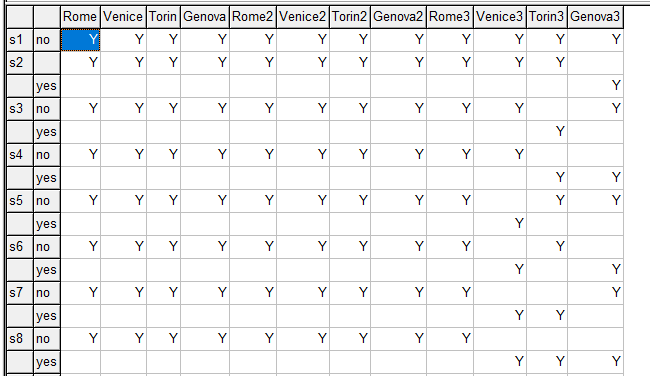
sets    i 'items' /Rome,Venice,Torin,Genova,Rome2,Venice2,               Torin2,Genova2,Rome3,Venice3,Torin3,Genova3 /    k 'objectives' /cost,hours,people,items/    s 'solution points' /s1*s4096/ ; * * check if set s is large enough * scalar size 'size needed for set s'; size = 2**card(i); abort$(card(s)'set s is too small',size; * * generate all combinations * sets   base 'used in next set' /no,yes/   ps0(s,i,base) / system.powersetRight /   ps(s,i) 'power set' ; ps(s,i) = ps0(s,i,'yes'); display ps;

The unusual construct system.powersetRight will populate set ps0 with information about the power set. I hardly ever use the Power Set, but there is a well-known formulation for the TSP (Traveling Salesman Problem), that can use this [3]. The generated set ps0 looks like (I pivoted things around to make the table a bit more readable):

ps0 with second index pivoted

This has a little bit more info than we need: we only need the "yes" rows. This "yes"-only part is stored in set ps. It looks like:

Set ps

It looks like we are missing solution s1 here. That is because GAMS stores everything sparse. A row without any Y elements is just not stored. The bottom of set ps looks like:

Bottom of set ps

Indeed we have all 4096 solutions (well, except for that funny first row).

1.2 Form our X parameters

With this we can form our \(x_{s,i}\in \{0,1\}\) parameter. We want a 0-1 parameter for two reasons: we want numerical values to evaluate our objectives, and we need this parameter later on to use a filter tool.

* * make a parameter out of this * parameter x(s,i) 'solutions'; x(s,i) = ps(s,i); * make sure row 1 exists: introduce an EPS x(s,i)$(ord(s)=1 and ord(i)=1) = eps; display x;

A trick to make the row not disappear is to insert an EPS value. An EPS value is like a zero when operated upon. But it exists: GAMS will no longer assume the whole row does not exist. 

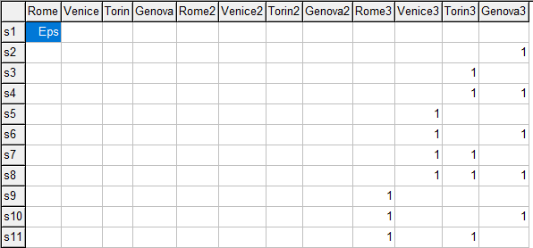Parameter x with EPS value

1.3 Form the F values

Now we have all possible solutions in the \(x\) space, we can start calculating the \(f\) values: the objectives. 

table data(i,k) '### data set with 12 items'              cost   hours  people     Rome     1000    5       5     Venice    200    1      10     Torin     500    3       2     Genova    700    7       8     Rome2    1020    5       6     Venice2   220    1      10     Torin2    520    3       2     Genova2   720    7       4     Rome3    1050    5       5     Venice3   250    1       8     Torin3    550    3       8     Genova3   750    7       8 ; data(i,'items') = 1; parameter f(s,k) 'objective values'; f(s,k) = sum(i, data(i,k)*x(s,i)); display f;

First we need to introduce our data. One objective is missing from the columns: the items. This is simply a column with ones: each item counts as one. With this we can calculate all \(f\) values in one swoop. The display output looks like:

----     56 PARAMETER f  objective values

             cost       hours      people       items

s1            EPS         EPS         EPS         EPS
s2        750.000       7.000       8.000       1.000
s3        550.000       3.000       8.000       1.000
s4       1300.000      10.000      16.000       2.000
s5        250.000       1.000       8.000       1.000
s6       1000.000       8.000      16.000       2.000
s7        800.000       4.000      16.000       2.000
s8       1550.000      11.000      24.000       3.000
s9       1050.000       5.000       5.000       1.000
s10      1800.000      12.000      13.000       2.000

. . . 

s4089    5930.000      37.000      52.000       9.000
s4090    6680.000      44.000      60.000      10.000
s4091    6480.000      40.000      60.000      10.000
s4092    7230.000      47.000      68.000      11.000
s4093    6180.000      38.000      60.000      10.000
s4094    6930.000      45.000      68.000      11.000
s4095    6730.000      41.000      68.000      11.000
s4096    7480.000      48.000      76.000      12.000

I only show the head and the tail of the display here. As we can see, some objective values violate the constraints. E.g. the last solution s4096, needs 76 people while we only have 50 available.

1.4 Constraint handling

We need to remove all solutions that violate the constraints. This can be done as follows:

parameter UpperLimit(k) 'bounds'/    cost 10000    hours  100    people  50 /; upperlimit(k)$(upperlimit(k)=0) = INF; set infeas(s) 'infeasible solutions'; infeas(s) = sum(k$(f(s,k)>UpperLimit(k)),1); scalar numfeas 'number of feasible solutions'; numfeas = card(s)-card(infeas); display numfeas; * kill solutions that are not feasible x(infeas,i) = 0; f(infeas,k) = 0;

This code removes all infeasible solutions from \(x\) and \(f\). Note that assigning a zero makes the corresponding records disappear: this is because GAMS stores everything sparse. The display shows:

----     71 PARAMETER numfeas              =     3473.000  number of feasible solutions

1.5 Filter out dominated solutions

In the result set there are quite a few dominated solutions. A solution \(f_1\) dominates \(f_2\) if:

1. All objectives are better or equal
2. There is one objective which is strictly better

Looking again at some of our solutions

----     87 PARAMETER f  objective values

             cost       hours      people       items

s1            EPS         EPS         EPS         EPS
s2        750.000       7.000       8.000       1.000
s3        550.000       3.000       8.000       1.000
s4       1300.000      10.000      16.000       2.000
s5        250.000       1.000       8.000       1.000
s6       1000.000       8.000      16.000       2.000
s7        800.000       4.000      16.000       2.000

we see that for this small subset

• s1 is non dominated 
• s5 dominates s2 and s3
• s7 dominates s4 and s6

Remember we are minimizing cost, hours and people while maximizing items. 

GAMS has a tool to filter large data sets, call mcfilter.

D:\projects>mcfilter No input file specified Usage: mcfilter xxx.gdx mcfilter will remove duplicate and dominated points in a multi-criteria solution set. The input is a gdx file with the following data:    parameter X(point, i):   Points containing binary values.                             If all zero for a point, use EPS.    parameter F(point, obj): Objectives for the points X.                             If all zero for a point, use EPS.    parameter S(obj):        Direction of each objective: 1=max,-1=min The output will be a gdx file called xxx_res.gdx with the same parameters but without duplicates and dominated points. D:\projects>

The X and the F parameters conform to our parameters. So the only thing to add are the signs of the objectives.

parameter sign(k) 'sign: -1:min, +1:max' /    (cost,hours,people) -1    items               +1 /; execute_unload "feassols",x,f,sign=s; execute "mcfilter feassols.gdx";

We see:

mcfilter v3.
Number of records     =     3473
Number of X variables =       12
Number of F variables =        4
Loading GDX data      =       15 ms
After X Filter, count =     3473
X Duplicate filter    =        0 ms
After F Filter, count =       83
F Dominance filter    =        0 ms
Writing GDX data      =        0 ms

There are 83 non-dominated or Pareto optimal solutions.

The final Pareto set looks like:

Non-dominated solutions

I list here the \(x\) values and the \(f\) values. As can be expected, a solution with all \(x_i=0\) is part of the Pareto set: doing nothing is very cheap; no other solution can beat this on price. Interestingly, project Genova3 is never selected.

Approach 2: use a series of MIP models

There is another way to generate these 83 points: use a MIP model. Or rather a series of MIP models. We use an algorithm like:

1. Generate an optimal MIP solution. If infeasible: STOP.
2. Add constraints: new solutions must be better in one objective
3. Go to step 1.

This approach will be shown in part 2.

Conclusion

We have described a small multi-objective problem. We established that:

• There are 4096 total combinations possible.
• After removing the infeasible solutions, there are 3473 solutions left.
• After removing the dominated solution, we are left with 83 Pareto optimal solutions. 

We used some less well-known GAMS tools in our script: a power set generator and a multi-criteria filter.

References

1. Best Combination Algorithm of Complex Data with Multiple Constraints, https://stackoverflow.com/questions/55514627/best-combination-algorithm-of-complex-data-with-multiple-contraints
2. Vilfredo Pareto, https://en.wikipedia.org/wiki/Vilfredo_Pareto
3. TSP Powerset Formulation, https://yetanothermathprogrammingconsultant.blogspot.com/2009/02/tsp-powerset-formulation.html

Math Checker?

Spell checkers are very useful. It may not be such a bad idea to have something like a "Math checker". It could flag things like:

References

1. Bashiri, M. & Karimi, H. J, Effective heuristics and meta-heuristics for the quadratic assignment problem with tuned parameters and analytical comparisons, J Ind Eng Int (2012) 8: 6. https://doi.org/10.1186/2251-712X-8-6