Friday, April 30, 2010

GAMS/GDX compression

In some cases GDX compression can make a lot of difference. Here are the results for a large CSV file:

File                                 Size
AccPsdData_2009-11-19Su.csv   594,332,819
AccPsdData_2009-11-19Su.gdx    24,765,003
AccPsdData_2009-11-19Su.gdx     4,318,222  (with compression turned on)

The CSV file was read using SQL2GMS:

--- Job readcsv.gms Start 04/28/10 15:50:32 WEX-WEI 23.3.3 x86_64/MS Windows    
GAMS Rev 233  Copyright (C) 1987-2009 GAMS Development. All rights reserved
Licensee: Erwin Kalvelagen                               G090213/0001CV-WIN
          Amsterdam Optimization Modeling Group                      DC4572
--- Starting compilation
--- readcsv.gms(69) 2 Mb
--- call =sql2gms.exe @sql2gms.txt
GDXIO.DLL version:GDX Library      Nov  1, 2009 23.3.3 WIN 14596.15043 VIS x86/MS Windows      
ADO version: 6.0
Query: select ComNam,CtrNam,VarNam25,Year,Value from [AccPsdData_2009-11-19Su.csv]
GDX id: AccPsdData (Parameter)
Number of rows: 3230069
Elapsed time: 113.29 seconds
Done
Query: select distinct ComNam from [AccPsdData_2009-11-19Su.csv]
GDX id: Com (Set)
Number of rows: 55
Elapsed time: 23.67 seconds
Done
Query: select distinct CtrNam from [AccPsdData_2009-11-19Su.csv]
GDX id: Ctr (Set)
Number of rows: 254
Elapsed time: 24.09 seconds
Done
Query: select distinct VarNam25 from [AccPsdData_2009-11-19Su.csv]
GDX id: Var (Set)
Number of rows: 50
Elapsed time: 23.93 seconds
Done
Query: select distinct Year from [AccPsdData_2009-11-19Su.csv]
GDX id: Year (Set)
Number of rows: 51
Elapsed time: 23.76 seconds
Done
--- readcsv.gms(96) 2 Mb
--- Starting execution - empty program
--- readcsv.gms(96) 2 Mb
*** Status: Normal completion
--- Job readcsv.gms Stop 04/28/10 15:54:03 elapsed 0:03:30.982

It is a little bit slow as we make different passes over the data. Probably this would be faster if it was stored in a database.

Note: the sets were created to make it easier to read the data in a GAMS model. This way we have sets that can be read during compile time and thus can be used as domain. It is easy to calculate those sets in GAMS at run time, but then they cannot be used as domains.

The compression was turned on by the statement:

* compress gdx file
$setenv GdxCompress 1

* execute conversion
$call =sql2gms.exe @sql2gms.txt

Thursday, April 22, 2010

Portfolio: from QP to LP

Someone asked me how to derive the LP in http://yetanothermathprogrammingconsultant.blogspot.com/2010/04/l1-portfolio-formulation.html from the standard QP formulation:

image

(see also http://www.or-exchange.com/questions/204/overview-of-portfolio-models).

Of course the first reference would be the original article:

Mean-Absolute Deviation Portfolio Optimization Model and Its Applications to Tokyo Stock Market,” Hiroshi Konno and Hiroaki Yamazaki, Management Science, Vol. 37, No. 5 (May, 1991), pp. 519-531 (http://www.jstor.org/pss/2632458)

However, here is simple, intuitive approach:

1. Form separable QP

First we plug in the definition of the covariances q(i,j), using:

image

Here the r’s are the returns at each t for each instrument i. The μ's are the means. This results in:

image

where

image

The a(i,t)’s are the mean adjusted returns.

2. Approximate by LP

Now it is easy to see how this can be approximated by an LP:

image

So the resulting L1 norm model looks like:

imageThe appropriate way to model the absolute value in this context was the subject of the discussion in http://yetanothermathprogrammingconsultant.blogspot.com/2010/04/l1-portfolio-formulation.html.

Monday, April 19, 2010

Generating all non-dominated solutions in a multi-objective integer programming model (II)

This is a simple algorithm to enumerate all (or a subset) of the efficient solutions of an integer programming problem. This is a slightly different approach than used in http://yetanothermathprogrammingconsultant.blogspot.com/2010/02/generating-all-non-dominated-solutions.html. Basically the algorithm is as follows:

  1. Choose any weights λi > 0
  2. repeat
    1. solve problem with weighted obj
    2. if infeasible: STOP
    3. record the efficient solution
    4. add cut to prevent this solution to be found again
    5. add constraint such that dominated solutions are not accepted

As example we use a simple model from J. Shapiro, “Multiple Criteria Public Investment Decision Making by Mixed Integer   Programming”, working paper, MIT, 1975:

max x1+10x2+9x3
max 10x1+x2+9x3
x1+x2+x3 ≤ 2
x1,x2,x3 ∈ {0,1}

The following GAMS model illustrates the algorithm on this small problem:

$ontext

  
Example (4) from

  
"Multiple Criteria Public Investment Decision Making by Mixed Integer
  
Programming", Jeremy F. Shapiro, WP 788-05, Alfred P. Sloan School of
  
Management, MIT, May 1975

  
erwin@amsterdamoptimization.com

$offtext


set j /v1,v2,v3/;
binary variables x(j);

set i /obj1,obj2/;
variables z(i),sz;
equations
   objs(i)
   e
   scalobj
;

parameter lambda(i);

table objcoeff(i,j)
       
v1  v2  v3
 
obj1   1  10   9
 
obj2  10   1   9
;

scalobj.. sz =e=
sum(i, lambda(i)*z(i));
objs(i).. z(i) =e=
sum(j, objcoeff(i,j)*x(j));
e..      
sum(j, x(j)) =L= 2;


*
* there are 7 feasible integer solutions
* here we calculate them all
*
equation edummy;
variable dummy;
edummy.. dummy=e=0;

set k/k1*k10/;
set dynk(k) 'dynamic set';
dynk(k) =
no;

equation cut(k);
parameter sol(k,j),obj(k,i);
sol(k,j) = 0;
cut(dynk).. 
sum(j, x(j)$(sol(dynk,j)>0.5) - x(j)$(sol(dynk,j)<0.5)) =l= sum(j$(sol(dynk,j)>0.5),1) - 1;

model m0 /edummy,e,objs,cut/;

option limrow=0, limcol=0;
m0.solprint=2;
m0.solvelink=2;

scalar ok/1/;
loop(k$ok,
  
solve m0 using mip minimizing dummy;
   ok = 1$(m0.modelstat=1
or m0.modelstat=8);
  
if (ok,
      dynk(k) =
yes;
      sol(k,j) = x.l(j);
      obj(k,i) = z.l(i);
   );
);

display "----------------------------------------------------",
       
" All solutions",
       
"----------------------------------------------------",
         sol,obj;


*
* calculate the min and max objectives
*
parameter minz(i), maxz(i);
model m1 /e,objs,scalobj/;
m1.solprint=2;
m1.solvelink=2;
alias (i,ii);
option optcr=0;
loop(ii,
    lambda(i) = 0;
    lambda(ii) = 1;
   
solve m1 using mip minimizing sz;
   
abort$(m1.modelstat<>1) "Not optimal";
    minz(ii) = sz.l;
   
solve m1 using mip maximizing sz;
   
abort$(m1.modelstat<>1) "Not optimal";
    maxz(ii) = sz.l;
);
display "----------------------------------------------------",
       
" Bounds for objectives",
       
"----------------------------------------------------",
         minz,maxz;

*
* calculate all efficient solutions
* this is a variation on the above:
* a new solution must be better in at least one obj than all previous
* solutions.
*

binary variable y(k,i);
equation nondom(k,i),ysum(k);

nondom(dynk,i)..  z(i) =g= obj(dynk,i) -  (maxz(i)-minz(i))*(1-y(dynk,i));
ysum(dynk)..     
sum(i,y(dynk,i)) =g= 1;


model m2 /e,objs,scalobj,cut,nondom,ysum/;
m2.solprint=2;
m2.solvelink=2;


obj(k,i) = 0;
sol(k,j) = 0;
dynk(k) =
no;

* any nonzero weight is ok.
lambda(i) = 1/
card(i);

ok=1;
loop(k$ok,
  
solve m2 using mip maximizing sz;
   ok = 1$(m2.modelstat=1
or m2.modelstat=8);
  
if (ok,
      dynk(k) =
yes;
      sol(k,j) = x.l(j);
      obj(k,i) = z.l(i);
   );
);

display "----------------------------------------------------",
       
" Efficient/nondominated solutions",
       
"----------------------------------------------------",
         sol,obj;


The first part is optional: we enumerate all feasible integer solutions. This is not possible for large problems, so in practice this step must be omitted. The results for this example:

----     73 ----------------------------------------------------
             All solutions
            ----------------------------------------------------

----     73 PARAMETER sol 

            v1          v2          v3

k2       1.000
k3       1.000       1.000
k4                   1.000
k5                               1.000
k6                   1.000       1.000
k7       1.000                   1.000

----     73 PARAMETER obj 

          obj1        obj2

k2       1.000      10.000
k3      11.000      11.000
k4      10.000       1.000
k5       9.000       9.000
k6      19.000      10.000
k7      10.000      19.000

So we have seven possible integer solutions. Note that solution k1 is v1=v2=v3=0, obj1=obj2=0. Many of them are dominated. E.g. solution k4 is dominated by solution k3 (note: we are maximizing).

In the model we need a big-M constant. To find good values for these constants we need to find the minimum and maximum values for each objective. That is done in part 2. The result is:

----     98 ----------------------------------------------------
             Bounds for objectives
            ----------------------------------------------------

----     98 PARAMETER minz 

                      ( ALL       0.000 )

----     98 PARAMETER maxz 

obj1 19.000,    obj2 19.000

This means we can use 19 as big-M value.

In the last part we enumerate all efficient or non-dominated solutions:

----    140 ----------------------------------------------------
             Efficient/nondominated solutions
            ----------------------------------------------------

----    140 PARAMETER sol 

            v1          v2          v3

k1       1.000                   1.000
k2                   1.000       1.000
k3       1.000       1.000

----    140 PARAMETER obj 

          obj1        obj2

k1      10.000      19.000
k2      19.000      10.000
k3      11.000      11.000

For very large problems we can make the set k sufficiently small so that we collect k non-dominated solutions instead of all possible non-dominated solutions. Note that the problem becomes larger and larger. The number of constraints added to the problem in each cycle is:

  • 1 cut to exclude this solution
  • (K+1) constraints to find non dominated solutions (here K is the number of objectives).

In addition we add each cycle K binary variables.

It is noted that the weights are not very important when we are able to find all efficient solutions. Just any nonzero weights will do.

Friday, April 16, 2010

Coin-or binaries

I was looking for a fresh CBC.EXE for Windows. But looking at this, Windows is not really popular here:

cbc

Thursday, April 15, 2010

mps –> GAMS

GAMS comes with a tool called mps2gms. With a large MPS file from a client I had some problems using this tool, and I spent some time to make it reproducible with a small example. The problem is related to a ranged equation:

NAME          Error
ROWS
N  obj
G  c1
E  c2
COLUMNS
    x1        obj                  1
    x1        c2                   1
    x2        c1                   1
    x2        c2                   1
RHS
    rhs       c1                  10
RANGES
    range     c1                   2
BOUNDS
FR bnd       x1
ENDATA

This model is like the following:

min x1
x1=−x2
10 ≤ x2 ≤ 12

The resulting GAMS model is complicated to look at with all data inside a GDX file. However when we run it against the CONVERT solver we can see the scalar GAMS version:

*  RMIP written by GAMS Convert at 04/15/10 19:04:26
*
*  Equation counts
*      Total        E        G        L        N        X        C
*          3        3        0        0        0        0        0
*
*  Variable counts
*                   x        b        i      s1s      s2s       sc       si
*      Total     cont   binary  integer     sos1     sos2    scont     sint
*          4        4        0        0        0        0        0        0
*  FX      0        0        0        0        0        0        0        0
*
*  Nonzero counts
*      Total    const       NL      DLL
*          6        6        0        0
*
*  Solve m using RMIP minimizing x1;


Variables  x1,x2,x3,x4;

Positive Variables  x3,x4;

Equations  e1,e2,e3;


e1..    x1 - x2 =E= 0;

e2..    x2 + x3 =E= 0;

e3..    x3 - x4 =E= 0;

* set non default bounds


* set non default levels


* set non default marginals


Model m / all /;

m.limrow=0; m.limcol=0;

Solve m using RMIP minimizing x1;

The constants 10 and 12 are not preserved and have disappeared from the model. I suspect that missing is x4.lo=10 and x4.up=12. (This is somewhat difficult to read as x1 and x4 are added to the model, and the mps columns x1 and x2 are renamed to GAMS variables x2 and x3). I have passed this on to GAMS for investigation so this can be fixed.

There was also another issue related to how the ranges section was read. In the end I used one of my own tools to quickly read in the mps file and write a GAMS file:

C:\projects\xxxxxx>\projects\lpsolve\lp2gams 2.mps
lp2gams.exe version 1.3
Erwin Kalvelagen, erwin@amsterdamoptimization.com

lp_solve version 5.5.0.11
Reading mps file 2.mps
Writing 2.gms
Rows: 5857   Columns: 4235   Nonzero elements: 19228
Done

C:\projects\xxxxx>

Update: the mps2gms issues are fixed for the next release.

Sunday, April 11, 2010

L1 portfolio formulation

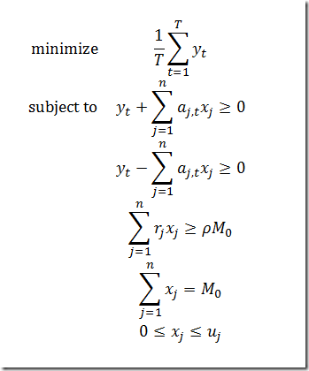
In the paper “Mean-Absolute Deviation Portfolio Optimization Model and Its Applications to Tokyo Stock Market,” Hiroshi Konno and Hiroaki Yamazaki, Management Science, Vol. 37, No. 5 (May, 1991), pp. 519-531 (http://www.jstor.org/pss/2632458) the following Linear Programming model is presented:

image

Here x(j) is the allocation (the variable we are interested in), and y(t) are auxiliary variables. The data are:

  • a(j,t) are mean adjusted returns
  • M0 is the budget
  • rho is the required return
  • r(j) are the stock returns

This model is in fact almost identical to what is presented in this blog before: http://yetanothermathprogrammingconsultant.blogspot.com/2009/07/ms-solver-foundation-excel-interface_07.html. Actually the formulation in the paper by Konno e.a. is slightly non-optimal: the big data block sum(j, a(j,t)*x(j)) is present twice in the model. For large data sets this can be felt in larger solution times. Hence a slightly better formulation could be:

imageOn a synthetic data set with n=2000 stocks and T=300 observations we have:

Model Konno ea Improved
variables 2300 2600
equations  602 302
nonzero elements 1,204,900 605,200
simplex iterations 2031 1224
solution time 8.9 2.97

GAMS/Gurobi did not really like my improved formulation:

Starting Gurobi...
Optimize a model with 302 Rows, 2600 Columns and 604600 NonZeros

Presolve time: 0.34s
Iteration    Objective       Primal Inf.    Dual Inf.      Time
       0    0.0000000e+00   1.320000e+00   0.000000e+00      0s
Out of memory
*** Out of memory
*** Could not solve problem (10001)

This is probably due to this 100% dense block. I’ll pass it on for investigation. Gurobi is under active development so this may be already working ok with later versions. To humble me it solves the original formulation from Konno/Yamazaki just fine!

The above timings were for Cplex/dual. As the original authors used MINOS, here are some timings with MINOS:

  • Konno e.a.: its:17032, time:28.7
  • Improved: its:11884, time:7.8

    The timings with Cplex/dual and Minos/primal point in the same direction. Note that MINOS is faster with the improved model than Cplex on the Konno model. So proper modeling can sometimes help more than choosing a faster solver (of course both having a better formulation and a faster solver is even better). The importance of proper modeling is usually more important for MIP models, but here we see some real differences in performance for different formulations in an LP.

  • Friday, April 9, 2010

    MIQP vs Dynamic Programming

    Looking at the posting http://thread.gmane.org/gmane.comp.lang.r.general/175564 I thought it should be possible to formulate this as a mathematic programming problem. The quadratic objective would yield an MIQP. An example formulation could be: http://amsterdamoptimization.com/models/blog/reading.gms. This is not really easy to solve. Even a MIP approximation (minimizing sum of absolute deviations) is not easy: http://amsterdamoptimization.com/models/blog/reading2.gms. Looks like we are loosing against dynamic programming here.

    Friday, April 2, 2010

    GAMS/Cplex: final solve can be expensive

    GAMS likes to display marginals on MIP models. It does this by solving an LP with all integers fixed at their current values. This final solve can be very expensive. Here is an example:

    ---   31,617 rows  92,289 columns  276,386 non-zeroes
    ---   128 discrete-columns


    Root relaxation solution time =    8.08 sec.

            Nodes                                         Cuts/
       Node  Left     Objective  IInf  Best Integer     Best Node    ItCnt     Gap

          0     0      154.2800     3                    154.2800    45818        
    *     0+    0                          154.2800      154.2800    45818    0.00%
          0     0        cutoff            154.2800      154.2800    45818    0.00%
    MIP status(101): integer optimal solution
                                                          
    B&B time: not displayed but estimated at < 1 sec
    Fixing integer variables, and solving final LP...
    Tried aggregator 1 time.
    LP Presolve eliminated 129 rows and 257 columns.
    Aggregator did 239 substitutions.
    Reduced LP has 31249 rows, 91793 columns, and 275012 nonzeros.
    Presolve time =    0.16 sec.
    Initializing dual steep norms . . .

    Iteration log . . .
    Iteration:     1   Dual objective     =             0.000000
    Perturbation started.
    Iteration:   102   Dual objective     =             0.000000
    Iteration:   538   Dual objective     =            13.863577
    Iteration:  1033   Dual objective     =            14.787416

    ….
    Iteration: 54455   Dual objective     =           151.954457
    Iteration: 54694   Dual objective     =           153.771165
    Iteration: 54911   Dual objective     =           153.771165
    Elapsed time =  188.09 sec. (55000 iterations).
    Iteration: 55190   Dual objective     =           153.771165
    Iteration: 55452   Dual objective     =           154.280180
    Removing perturbation.
    Fixed MIP status(1): optimal  
                                                           Final LP: time not displayed but estimated at > 188 sec

    So we have approximately:

    1. Root LP: 8 sec
    2. B&B: 1 sec
    3. Final LP: 188 sec

    If we are not interested in duals (for most MIP models this is the case), the last step be omitted with an option (SOLVEFINAL=0). That would reduce the total solution time from 200 seconds to 10 seconds.

    Only the root time is displayed, so I had to guess the other times.