Linearizations in a Land-Use Planning Model

There are often multiple ways to formulate a problem. With a modeling language it is easy to try out quickly different formulations. This can have a significant effect on the performance of the model.

Problem description

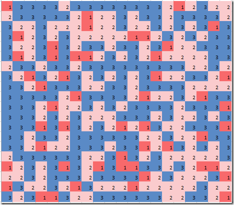
Assuming a grid of cells (plots) we want to assign plots to a certain land use. Each plot has different development cost for different cells. This is much like an assignment problem. Each plot is assigned to a single land-use type and the total area to be assigned to each land-use type is given. Below is an example of a solution if we minimize the total cost using random cost coefficients on a 20 x 20 grid with three land-use types:

This assignment is in practice not very good: we also require some clustering or compactness. Here is a solution where we use a composite objective function with a cost component and a compactness component:

Problem set up

This problem requires just a few sets and some data. The cost data is randomly generated.

MINLP/MIQCP Model

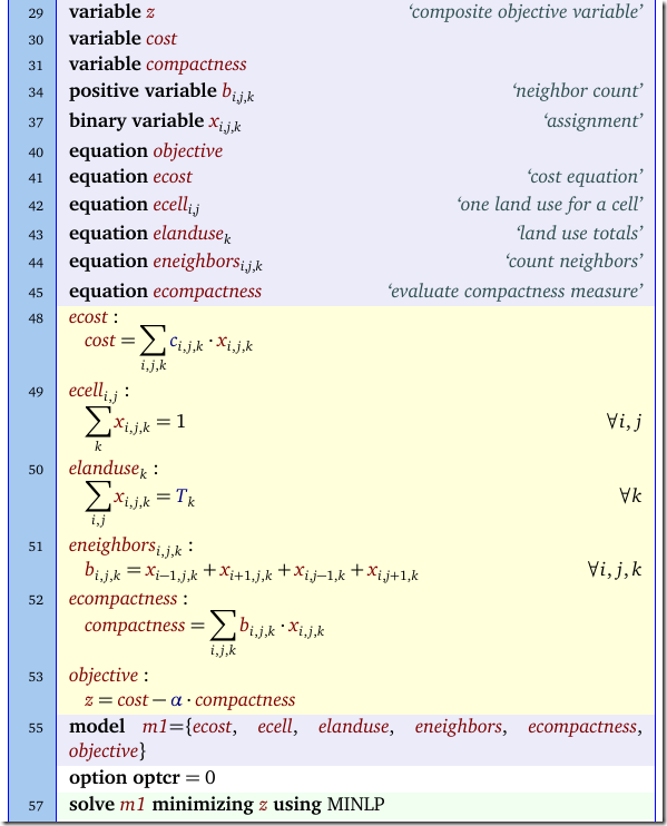
The MINLP model for this problem can look like:

The interesting part is how the compactness is expressed. Basically a plot gets more weight if the cell and its neighbors have the same land use type. The equations eneighbors and ecompactness take care of this. Unfortunately in equation ecompactness we multiply two variables resulting in a MINLP model. Looking at the nature of the non-linearities we can see they are quadratic. This makes it possible to use solvers like Cplex and Gurobi to solve this.

Linearization I

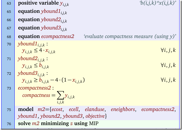
In the paper by Aerts e.a. the following linearization is suggested:

In the paper the variable b is substituted out, but I rather keep it in the model.

Linearization II

Here I propose a different linearization. Instead of linearizing the expression

 

it may be useful to linearize the components:

 

We can do this as follows:

We added some complexity here: the offset parameter indicates the lead (+1) and lags (-1) on the indices i and j. Once we have this offset parameter correctly set up we can deal with these four different binary multiplications in one swoop, using the familiar:

Linearization III

When we take the objective into account, we can see we actually can drop equation gambound3 from the last model. The reason is that the model will automatically try to push the values for Γ upwards (we are minimizing –Γ). So our next version of the model would be:

Linearization IV

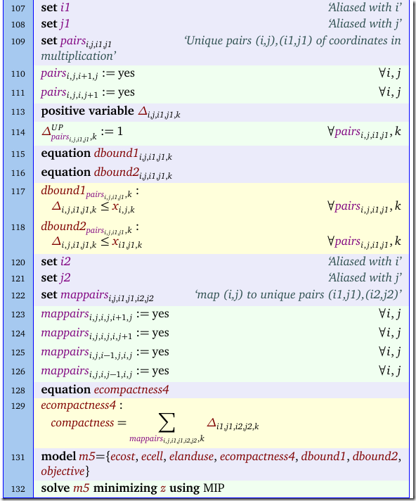
There is further improvement possible by considering that we are repeating some binary multiplications. When considering cell (2,2) we use x(2,3)*x(2,2) and when considering cell (2,3) we look at x(2,2)*x(2,3). However these are the same. Keeping track which pairs we already considered is an interesting exercise.

Here is one approach where we use extra sets to do some bookkeeping.

Performance

In some cases the last formulation is much better (all timings in seconds using one thread):

Model	Solver	Objective	Solve Time	Nodes	Equations/Variables	Notes
MIQCP	Gurobi	-220.5441	20	105	1,606/2,403	ecompactness rewritten as ≤ constraint.
MIP I	Gurobi	-220.5441	31	171	5,206/3,603
MIP II	Gurobi	-220.5441	5	0	14,806/6,003
MIP III	Gurobi	-220.5441	3	0	10,006/6,003
MIP IV	Gurobi	-220.5441	2	0	4,966/3,483

Gurobi is really helped by using the new linearization: it does not need to do any work in the branch-and-bound but rather solves everything during preprocessing (as indicated by a node count of zero). Note that models MIP II and III are doing very good but are also the largest (using number of equations and variables as a measure). Again we see that the size of a model is not always a good indicator for how difficult the model is.

(Note: Baron is actually doing very good on the MINLP model: 30 seconds).

Results with Cplex (8 threads):

Model	Solver	Objective	Solve Time	Nodes	Equations/Variables	Notes
MIQCP	Cplex	-220.5441	30	2087	1,606/2,403	ecompactness rewritten as = constraint.
MIP I	Cplex	-220.5441	10	39	5,206/3,603
MIP II	Cplex	-220.5441	5	0	14,806/6,003
MIP III	Cplex	-220.5441	3	0	10,006/6,003
MIP IV	Cplex	-220.5441	2	0	4,966/3,483

The same pattern emerges. As expected, throwing extra threads at a model that only needs zero nodes, does not really help.

Notes

• We cannot solve exactly the same model with Gurobi and Cplex. We need to change the sign of the ecompactness constraint. I do not completely understand this right now.
• Reformulations can be  more powerful than faster hardware.
• The performance of different formulations is often difficult to predict. The best way to evaluate is just to implement them. A high level modeling language can help here tremendously.
• Just working on different formulation may lead to ideas about further improvements.
• The original MINLP model may serve as the “logical design” while the best linearization could be called the “physical model”. 
• We used random values for c(i,j,k). This may make the solution of the problem easier than using real data which may have fewer different values and show more structured patterns. These real-world data sets have more symmetry and less differentiation in cost which can hinder a branch-and-bound solver.