Wednesday, March 23, 2016

ggplot and miptrace

The output of miptrace can be used to plot the MIP bounds. In this post we used it to show the results on an Exam Scheduling Model. After a little bit of clean-up here is a better version:

plot.trace <- function(filename,ylimits,title=basename(filename)) {
  hdr<-c("lineNum", "seriesID", "node", "Seconds", "bnd1", "bnd2")
  df<-read.csv(filename,na.strings = " na",header=F,comment.char="*",col.names=hdr)
  library(tidyr)
  df<-gather(df,key=bound,value=Objective,bnd1,bnd2)
  p<-ggplot(data=df,aes(x=Seconds))+geom_line(aes(y=Objective,color=bound),size=1.03)+
    ggtitle(title)+theme(legend.position=c(.8, .8))+
    scale_color_manual(name="MIP Bounds",values=c("blue","red"),
                       labels=c("Best Found Integer Solution","Best Possible Integer Solution"))
  if (!missing(ylimits)) {
    p<-p+ylim(ylimits)
  }
  return(p)
}
plot.trace("c:/tmp/exam3.csv",c(0,2000),"Exam Scheduling MIP Model")

We pivot the data into long format (“collapsing” the last two columns with the bounds into a key, value pair of columns). The output looks like:

image

Monday, March 21, 2016

Exam scheduling: Debugging C++ vs Modeling

In this post a question was asked about a small interesting scheduling problem. The model was implemented in C++ using Cplex. Debugging someone else’s C++ code is not my favorite pastime so instead just lets implement the model in a modeling language (that also is probably faster than staring at some C++ code).

We have 10 time slots (two per day). We want to assign 59 different exams to time slots such that students that do multiple exams are not burdened more than needed. We have some data indicating conflicts: for exam pairs \((i,j)\) (with \(i<j\)) we have the number of students that want to take both exams. This number is called \(\mathit{conflicts}_{i,j}\).

image 

This matrix is strictly upper-triangular. In the above picture there are some apparent sub-diagonal elements but that is a visual aberration. This is the result from dropping rows and columns without entries. The central binary variable is:

\[x_{i,t} = \begin{cases} 1 & \text{if exam $i$ is taken at period $t$} \\
                                   0 & \text{otherwise}
\end{cases}\]

The hard constraints are as follows: each exam is offered exactly one time, and exams with conflicts cannot be offered at the same time. These are the easy ones:

image

The soft constraints are:
  1. A penalty of 6 for each student that has two exams on one day.
  2. A penalty of 1 for each student with exams on two consecutive days.
  3. A penalty of 2 for each student with an afternoon exam followed by morning exam the next day.

All these penalties are based on a similar concept: count the conflicts. This counting is done as follows:

image

Here the variables yd, yd2 and yd3 are binary variables (although they can be relaxed to continuous variables between zero and one). We can just use a lower bound as we are minimizing those counts. The sets dt1, dt2 and dt3 indicate the periods to consider. E.g. dt1 looks like:

image

dt2 is:

image

dt3 is a subset of dt2:

image

The objective is to minimize the penalties on the conflicts:

image

The final model solves quite reasonably with Cplex:

exam3

Here the blue line is the objective (best found) and the red line is the lower bound (best possible). We see that Cplex finds good solutions quickly but needs more time to prove optimality. To get good performance I helped Cplex a little bit with setting branching priorities and using some options suggested by a tuning run.

Note: the plot was produced by the GAMS/Cplex option miptrace and some R code:

> ggplot(data=exam,aes(x=seconds))+geom_line(aes(y=bestFound),color="blue",size=1.1)+
+     geom_line(aes(y=(bestBound)),color="red")+ylim(0,500)+ylab("objective")

The results look like:

exam3

Here, we allocated penalties for a conflict \((i,j)\) to \(i\). Note that it would be easy to add a capacity constraint where we would limit the number of parallel exams in each time period. The would prevent the uneven distribution of exams over the time periods.

The conflicts are numerous. We have 14 same day conflicts;

image

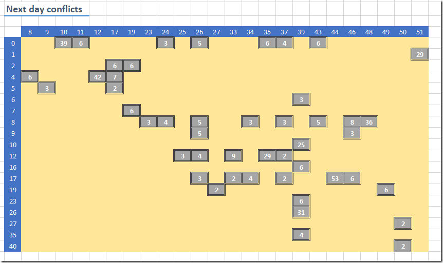
The solution has further a lot of next day conflicts (although it is able to circumvent the ones with a really high student count).
image

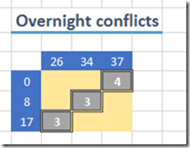
There are just a few overnight conflicts:
image

Note that these come in addition to the next day conflicts. The total of these (where we apply given penalties) result in our optimal objective:

image

In my opinion it is much more convenient to develop models in a modeling language as this will allow you to think and reason better about the model equations and to make quick changes to the model. Once that is working you can always translate these constructs into C++ or other programming languages.

Wednesday, March 16, 2016

Large assignment problem

I usually solve assignment problems:

\[\begin{align} \min\>& \sum_{i,j} c_{i,j} x_{i,j} & \\ & \sum_j x_{i,j} = 1 & \forall i \\ & \sum_i x_{i,j} = 1 & \forall j \\ & x \in \{0,1\} \end{align}\]

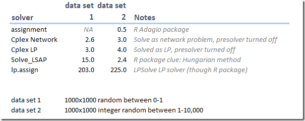
as an LP or MIP. It is often argued that specialized solvers are much faster on this. Here some results with a \(1000\times 1000\) problem, artificially created:

image

See also here. One of the advantages of using an LP/MIP is that I can react more quickly on changes in the problem. Often what starts out as a straight assignment problem becomes in the end something rather different. See here for an example of that.

Notes:

  • The assignment solver in the R Adagio package deals with integer cost coefficients only.
  • Current state-of-the art LP solvers are very, very fast. The need for specialized network solvers in these packages becomes somewhat less apparent. Indeed Gurobi does not offer one.
  • lp.assign is just calling the LPSolve LP/MIP solver.

Saturday, March 12, 2016

R: is.integer and is.wholenumber

It is not the first time that a user is confused with this R output:

> is.integer(1)
[1] FALSE

The reason is the type of such a number is actually:

> typeof(1)
[1] "double"

The help of is.integer is actually doing a good job of pointing this out. However in this help an interesting suggestion is made for a function is.wholenumber. The purpose of this function is to check if the value of a number (opposed to the type) is an integer:

> is.wholenumber <-
+
    function(x, tol = .Machine$double.eps^0.5)  abs(x - round(x)) < tol
>
is.wholenumber(1)
[1] TRUE

Now the question is: why this tolerance of \(\sqrt{\epsilon}\)?

I probably would have implemented this function with the more naïve:

> my.is.wholenumber <- function(x) x==round(x)

i.e. use a tolerance of zero. May be a tolerance equal to the machine precision .Machine$double.eps could be useful (I am not sure of that), but a tolerance of \(\sqrt{\epsilon}\)?  I came up with this hypothesis. \(\epsilon\approx \)1.0e-16 so about 15 decimal places. The square root of this is about 7 decimal places. The default number of decimals in a print statement is 7:

> .Machine$double.eps
[1] 2.220446e-16
>
.Options$digits
[1] 7

So may be the goal was to keep the print precision and the behavior of is.wholenumber in sync:

> 1.000005
[1] 1.000005
> 1.0000000005
[1] 1
> is.wholenumber(1.000005)
[1] FALSE
> is.wholenumber(1.0000000005)
[1] TRUE

It does not work perfectly:

> 1.00000005
[1] 1
>
is.wholenumber(1.00000005)
[1] FALSE

Any better explanations around?

Friday, March 11, 2016

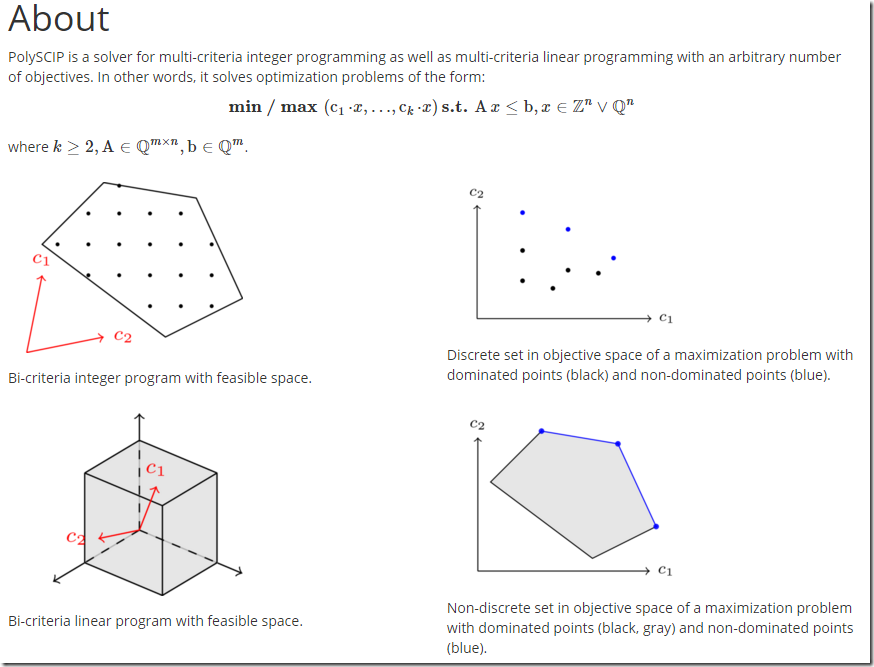
PolySCIP: multi-criteria integer programming

http://polyscip.zib.de/

image

Looks interesting. Unfortunately, not being an academic I am not allowed to download it and try it out.

GAMS/Gurobi Announcement

Received from sales@gams.com:

Next week we will start to release the distribution 24.7.

There is one change, which will also affect your clients using GAMS/Gurobi: Gurobi Optimization, Inc. has decided to end the current arrangement that allows us to offer GAMS/Gurobi integrated licenses. Thus we will no longer be able to sell new or upgrade (e.g. enlarge a single user license to a 5 user license) existing GAMS/Gurobi licenses after March 19, 2016. Existing license are (sic) perpetual and will continue to work with your current GAMS distribution.

However, to maintain access to upcoming versions of GAMS/Gurobi, Gurobi Optimization, Inc. requires that commercial GAMS/Gurobi licenses are kept under maintenance. If the maintenance for a commercial GAMS/Gurobi license has expired, it must be renewed before the end of April 2016.
If an academic GAMS/Gurobi user wants to renew maintenance, we will be downgrade (sic) the license for GAMS/Gurobi to a GAMS/Gurobi-link license and he will have to get a Gurobi license directly from Gurobi, Gurobi Optimization Inc.

For details and further information please consult the release notes for 24.7 at: 
http://www.gams.com/help_beta/topic/gams.doc/releasenotes/24.7.html#g2470_GUROBI

This will make it more cumbersome to evaluate GAMS/Gurobi against other MIP solvers and to procure and use GAMS/Gurobi. Looks to me like a lose-lose-lose proposition for both GAMS, Gurobi and the customer. I guess at least someone must look at this differently than I do.

Meanwhile in twitter space:

image

Microsoft: Python, R

Python 3 starts to take over Python 2 (finally!)

pypi-chart-2

An analysis by Microsoft looking at packages requiring Python 2 or Python 3, gives an indication when Python 3 starts to take over: that is when more packages work with 3 than with 2. Conclusion: In 3 months, Python 3 will be better supported than Python 2.

Links:

R Tools for Visual Studio

RTVS-1

Looks very much like RStudio.

Links:

Tuesday, March 8, 2016

MIP vs Matlab

In this post an interesting problem is posted. Too bad there is little or no background given on this problem. I am trying to suggest an optimization model opposed to some heuristic algorithm in Matlab. Looking at the zero points I get for my answer, without much success. I still think the MIP model is rather elegant. Here is the problem:

image

We have a large matrix with 10 columns and around 250k rows. The values are –1 and +1. We need to select N rows such that if we add up the columns of the selected rows, the average of the absolute values of those sums is minimized.

We can formulate this as very large MIP model with about 250k binary variables indicating if a row is selected.

There is however a data trick we can use. Observe that each cell has two possibilities, so there are only 2^10=1024 different possible rows. Our data is now essentially a fixed 1024 x 10 matrix and a vector of length 1024 of counts that tell us how many rows of each type we saw.

image

Now we only have to use 1024 integer variables. The upper bounds on the integer variables are the counts. Actually we can tighten that a little bit: it is the minimum of the count and N. The complete MIP model can look like:

250

We use a traditional variable splitting technique to model the absolute value. Note also that instead of the average or mean we just minimize the sum.

To test this formulation first we need to generate this 1,024 row matrix. In GAMS you can do this as follows:

set
  i
/n1*n1024/
  j
/j1*j10/
  val
/ '-1','+1'/
  ps(i,j,val)
/ system.PowerSetRight /
;

parameter a(i,j);
a(i,j)$ps(i,j,
'+1'
)=1;
a(i,j)$ps(i,j,
'-1'
)=-1;

The set ps is populated with:

image

Using this set, we form the parameter a as follows:

image

This is exactly the format we are looking for.

For some large values for N, the MIP solver will solve this problem surprisingly fast. Here is a log with the open source solver CBC:

COIN-OR Branch and Cut (CBC Library 2.8)
written by J. Forrest

Calling CBC main solution routine...
Integer solution of 6 found by DiveCoefficient after 0 iterations and 0 nodes (0.06 seconds)
Integer solution of 4 found by RINS after 0 iterations and 0 nodes (0.07 seconds)
Integer solution of 0 found by DiveCoefficient after 1 iterations and 0 nodes (0.15 seconds)
1 added rows had average density of 992
At root node, 1 cuts changed objective from 0 to 0 in 2 passes
Cut generator 0 (Probing) - 0 row cuts average 0.0 elements, 1 column cuts (1 active)  in 0.002 seconds - new frequency is 1
Cut generator 1 (Gomory) - 9 row cuts average 928.6 elements, 0 column cuts (1 active)  in 0.004 seconds - new frequency is -100
Cut generator 2 (Knapsack) - 0 row cuts average 0.0 elements, 0 column cuts (0 active)  in 0.000 seconds - new frequency is -100
Cut generator 3 (Clique) - 0 row cuts average 0.0 elements, 0 column cuts (0 active)  in 0.000 seconds - new frequency is -100
Cut generator 4 (MixedIntegerRounding2) - 0 row cuts average 0.0 elements, 0 column cuts (0 active)  in 0.001 seconds - new frequency is -100
Search completed - best objective 0, took 1 iterations and 0 nodes (0.15 seconds)
Maximum depth 0, 0 variables fixed on reduced cost

Solved to optimality.
MIP solution:   0.000000e+000   (0 nodes, 0.171 seconds)

Very impressive results (other good MIP solvers perform similar).

Sunday, March 6, 2016

The Weight Problem of Bachet de Meziriac

In a comment in this post there was a question about the Weight Problem of Bachet de Meziriac.

From this description:

A merchant had a forty pound weight that broke into four pieces as a result of a fall. When the pieces were subsequently weighed, it was found that the weight of each piece was a whole number of pounds and that the four pieces could be used to weigh every integer weight between 1 and 40 pounds. What were the weights of the pieces?

This problem comes from the French mathematician Claude Gaspard Bachet de Méziriac (1581-1638) who solved it in his famous book Problèmes plaisants et délectables qui se font par les nombres, published in 1624.

We assume a balance scale where we can place weights in the  left or right pan like:

Photo by Nikodem Nijaki (Own work) [CC BY-SA 3.0], via Wikimedia Commons

MINLP formulation

A first simple MINLP formulation can look like:

image

The variable \(\delta_{i,k} \in \{-1,0,+1\}\) indicates whether we place the weight \(i\) on the left or the right scale during trial \(k\). Of course the equation Check is non-linear, so we need to solve this with a MINLP solver. The non-convexity we introduced requires a global MINLP solver such as Baron or Couenne. This formulation is probably similar to how one would formulate things for use with a Constraint Programming solver.

CP (Constraint Programming) formulation

Indeed a CP formulation in Minizinc can be found on Paul Rubins blog. CP solvers typically have no problem with many types of non-linearities as long everything stays integer-valued (CP solvers have limited support for continuous variables).

MIP formulation

It is not too difficult to make a MIP model from this. The linearization of the multiplication of a binary variable times a continuous variable is well known: 

\[ \boxed{\begin{align}&y= \delta \cdot x\\ &\delta\in\{0,1\}, x\ge 0 \end{align}}\] \[\>\>\Longleftrightarrow\>\>\] \[\boxed{\begin{align} & y\le \delta M\\ & y\le x\\ & y\ge x-M(1-\delta)\\ & \delta \in\{0,1\},x,y \ge 0 \end{align}}\]

Here \(M\) is a tight upper-bound on \(x\).

Instead of \(\delta_{i,k} \in \{-1,0,+1\}\) we now use \(\delta_{i,k,lr} \in \{0,1\}\) where \(lr=\{left,right\}\). We don’t want to place the same weight on the left and right scale, so we add the constraint \(\delta_{i,k,’left’}+\delta_{i,k,’right’}\le 1\). Note that this constraint is not really needed: the final result would not change if we left this constraint out.  Here are the changes to the model:

image

We also added the Order constraint: \(x_{i+1}\le x_i\). This gives a nicer display of the results but also reduces symmetry. This can make large models (much) easier to solve.

Results

The final result is:

----     40 VARIABLE x.L  the four weights

w1 27,    w2  9,    w3  3,    w4  1

The MINLP solvers Baron and Couenne do actually pretty good on the MINLP version of this model.

Friday, March 4, 2016

Reformulate MINLP to MIP

In this post the question came up, what type of solver can handle this problem:

\[\begin{align} \max\> & (0.9 x_0 + 0.8 x_1 + 0.85 x_2) \cdot(0.95 x_3 + 0.8 x_4 + 0.7 x_5)\cdot (0.98 x_6 + 0.94 x_7) \\ & x_0 + x_1 + x_2 = 1\\ & x_3 + x_4 + x_5 = 1 \\ & x_6 + x_7 = 1\\ & 3 x_0 + x_1 + 2 x_2 + 3 x_3 + 2 x_4 + x_5 + 3 x_6 + 2 x_7 \le 6 \\ & x_i \in \{0,1\} \end{align}\]

This is a non-linear model with integer restrictions: the objective is nonlinear and the equations are all linear. The first inclination would be to use a MINLP solver. However, because all products involve only binary variables, this model is easily linearized. The idea is that \(y=x_1\cdot x_2\cdot x_3\) with \(x_i\in\{0,1\}\) is equivalent to a set of linear inequalities :

\[ \boxed{\begin{align}&y=x_1\cdot x_2\cdot x_3\\ &x_i\in\{0,1\} \end{align}}\] \[\>\>\Longleftrightarrow\>\>\] \[\boxed{\begin{align} &y\le x_1\\ &y\le x_2\\ &y\le x_3\\ &y\ge x_1+x_2+x_3-2 \\ &y\in\{0,1\},x_i\in\{0,1\} \end{align}}\]
This is so tight we can even relax the integer restriction on \(y\) to \(y \in [0,1]\).

This means we can reformulate the MINLP model to a linear MIP model. For the full model we have:

\[\begin{align} \max\>\>& 0.9 \cdot 0.95 \cdot (0.98 y_{036} + 0.94 y_{037}) +\\ & 0.9 \cdot 0.8 \cdot (0.98 y_{046} + 0.94 y_{047}) +\\ & 0.9 \cdot 0.7 \cdot (0.98 y_{056} + 0.94 y_{057}) +\\ & 0.8 \cdot 0.95 \cdot (0.98 y_{136} + 0.94 y_{137}) +\\ & 0.8 \cdot 0.8 \cdot (0.98 y_{146} + 0.94 y_{147}) +\\ & 0.8 \cdot 0.7 \cdot (0.98 y_{156} + 0.94 y_{157}) +\\ & 0.85 \cdot 0.95\cdot (0.98 y_{236} + 0.94 y_{237}) +\\ & 0.85 \cdot 0.8 \cdot (0.98 y_{246} + 0.94 y_{247}) +\\ & 0.85 \cdot 0.7 \cdot (0.98 y_{256} + 0.94 y_{257}) \\ \text{s.t.}\>\> & y_{036} \le x_0, \> y_{036} \le x_3, \> y_{036} \le x_6 \\ &y_{037} \le x_0, \> y_{037} \le x_3, \> y_{037} \le x_7 \\ &y_{046} \le x_0, \> y_{046} \le x_4, \> y_{046} \le x_6 \\ &y_{047} \le x_0, \> y_{047} \le x_4, \> y_{047} \le x_7 \\ &y_{056} \le x_0, \> y_{056} \le x_5, \> y_{056} \le x_6 \\ &y_{057} \le x_0, \> y_{057} \le x_5, \> y_{057} \le x_7 \\ &y_{136} \le x_1, \> y_{136} \le x_3, \> y_{136} \le x_6 \\ &y_{137} \le x_1, \> y_{137} \le x_3, \> y_{137} \le x_7 \\ &y_{146} \le x_1, \> y_{146} \le x_4, \> y_{146} \le x_6 \\ &y_{147} \le x_1, \> y_{147} \le x_4, \> y_{147} \le x_7 \\ &y_{156} \le x_1, \> y_{156} \le x_5, \> y_{156} \le x_6 \\ &y_{157} \le x_1, \> y_{157} \le x_5, \> y_{157} \le x_7 \\ &y_{236} \le x_2, \> y_{236} \le x_3, \> y_{236} \le x_6 \\ &y_{237} \le x_2, \> y_{237} \le x_3, \> y_{237} \le x_7 \\ &y_{246} \le x_2, \> y_{246} \le x_4, \> y_{246} \le x_6 \\ &y_{247} \le x_2, \> y_{247} \le x_4, \> y_{247} \le x_7 \\ &y_{256} \le x_2, \> y_{256} \le x_5, \> y_{256} \le x_6 \\ &y_{257} \le x_2, \> y_{257} \le x_5, \> y_{257} \le x_7 \\ & x_0 + x_1 + x_2 = 1\\ & x_3 + x_4 + x_5 = 1 \\ & x_6 + x_7 = 1\\ & 3 x_0 + x_1 + 2 x_2 + 3 x_3 + 2 x_4 + x_5 + 3 x_6 + 2 x_7 \le 6 \\ & x_i \in \{0,1\} \\ & y_{i,j,k} \in [0,1] \\ \end{align}\]

Notice that we dropped the \(\ge\) inequalities in the linearization. That is not by accident. We can leave them out as we are maximizing and pushing each \(y\) upwards.

Conclusion: MINLP models can save you a lot of typing.

Could a modeling system like GAMS help with this expansion? Well yes. We can let GAMS do the heavy lifting of the expansion as follows:

set i /i0*i7/;
alias
(i,j,k);
set cp(i,j,k) 'cross-products' /

  
(i0,i1,i2).(i3,i4,i5).(i6,i7)
/;

This would allow us to write:

objective.. z =e= sum(cp(i,j,k), c(i)*c(j)*c(k)*y(i,j,k));
linearize1(cp(i,j,k)).. y(i,j,k) =l= x(i);
linearize2(cp(i,j,k)).. y(i,j,k) =l= x(j);
linearize3(cp(i,j,k)).. y(i,j,k) =l= x(k);

Thursday, March 3, 2016

More Tennis Scheduling

Consider the case where we want to design a mixed doubles tennis tournament. Mixed doubles means every team consist of one man and one woman. The idea is to have several rounds where we want try to to have players with and against many different players. We implement this by forbidding to play with another person more than once, and also forbid to play against another player more than once. An additional goal is to have teams of the same strength play against each other. I.e. we don’t want a very strong team play against a very weak team. This we do by minimizing the differences in team ratings. 

Some data:

image 

To summarize:

  • We have 12 players: 6 male and 6 female.
  • We have 3 rounds with 3 games (so 3 courts). So in each round we have 6 teams.
  • Each player has a rating. For this exercise we just invent them using random numbers drawn from a uniform distribution.

We have a bunch of decision variables:

image

The central variable is team. This is binary variable indicating player \(p\) is assigned to team \(t\) during round \(r\). The derived variable game is integer valued automatically, so we declare it as just positive and set its upper bound to one. (It is not always clear this is a good approach – in some cases it is better just to declare as binary).

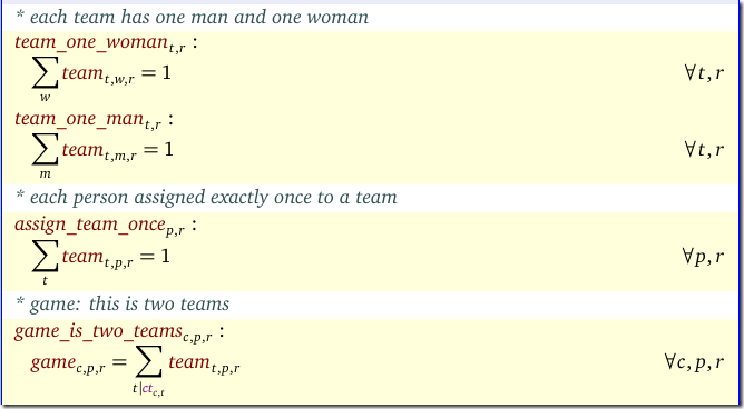
The first equations are easy:

image

In the last equation the \(ct_{c,t}\) mapping helps to find the two teams that play on court \(c\).  The first two constraints should probably be rewritten as a single constraint using an extra set \(gender=\{male,female\}\).

The other equations in the model deal with:

  • “play with” constraints.
  • “play against” constraints. These two are essentially the result of a linearization of a product of binary variables.
  • Ratings constraints.
  • Anti-symmetry constraints. We can add some additional constraints to reduce the symmetry in the model.

The results look like:

image

Tennis Scheduling

Scheduling models are not always simple to write down. Here someone is quite stuck in the mud trying to implement a scheduling model in the Constraint Programming system Choco. Let’s see if some Math Programming can do the job.

This is what we know:

image

So:

  • We have 12 time periods
  • We have three courts
  • We have 8 players
  • We have some data about forbidden assignments of players to slots
  • A game uses two (consecutive) time slots

Here is my MIQCP model:

tennis2

It has one non-linear (quadratic) equation: Twoslots1. However this is a binary multiplication, so we can easily linearize this using the familiar construct:

\[\begin{align}&g_{p,c,t} \le x_{p,c,t}\\ &g_{p,c,t} \le x_{p,c,t+1}\\&g_{p,c,t} \ge x_{p,c,t}+x_{p,c,t+1}-1 \end{align}\]

Now we have a straight MIP model. We try to prevent someone playing very few games, so we maximize the minimum number of games a person plays. The final results look like:

tennis2a

The red cells indicate: not allowed. Otherwise the numbers in the cells represent the tennis-court.

Wednesday, March 2, 2016

Ceiling function in a Mixed Integer Program

In this post the question was asked how to implement the Ceiling() function in a MIP model. The constraint in question is:

\[\left\lceil \frac{x-A}{B} \right\rceil \cdot C + D\cdot x < E \]

Answer:

Introduce an integer variable \(y\) and a continuous slack variable \(s\) and write:

\[\begin{align} &y\cdot C + D \cdot x \le E\\ &y=\frac{x-A}{B} + s\\ &s \in [0, 0.999]\\ &y \in \{\dots,-3,-2,-1,0,1,2,3,\dots\}\end{align}\]

Note that \(<\) constraints are no good, so make that \(\le\). We have a very small area for \(s\) that we don’t allow: between 0.999 and 1. This is to prevent that the ceiling of an integer \(k\) is the next integer \(k+1\).