Wednesday, October 31, 2012

GAMS and MsgBox

It is remarkably difficult to show a Windows message box in GAMS and react on it at execution time:

$onecho > q.vbs
Select Case MsgBox("No data for ID=" & WScript.Arguments.Item(0) & " Continue?",4,"Database Error")

Case vbYes
   
returnValue = 1
Case vbNo
   
returnValue = 0
End Select
WScript.Quit(returnValue)
$offecho


set
  errorID(*) 
'dynamic set with error IDs'
;

* assume we have an error
errorID(
'myErrorId') = yes;

scalars

   rc
'return code' /0/
   first
/1/
;


* I don't want to put out anything, but this $%!%@$$#! put_utility requires it
file dummy /xx/;
put
dummy;

loop
(errorID$first,
  
put_utility 'exec' / 'cscript //nologo q.vbs '
errorID.tl;
   rc = ErrorLevel;
   first=0;
);


display
rc;

I always cringe when I need to use this dreaded put_utility.

Background: in theory database systems can be designed such that data is always consistent. In practice almost all databases contain data problems. Somehow when doing optimization models we hit these errors more often than other db applications. This code is related to a larger model where we need to react on detecting some form of db error, i.e. stop or try to fix and continue.

image

Monday, October 29, 2012

Notation

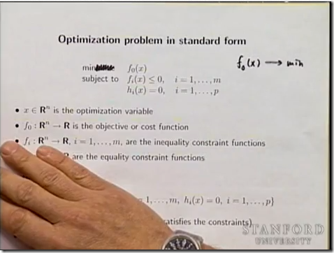
In http://www.youtube.com/watch?v=Ry5i8DGZrJs&list=EC3940DD956CDF0622&index=5&feature=plpp_video (approx. 2nd minute), Stephen Boyd says we are not allowed to use the notation:

image

It should be:

image

I guess I am somewhat of a repeat offender (I use the “min” notation a lot, “such that” not so much). The argument has to do with the English language. Apparently the Russian notation

imageis allowed (why can they use “min” and I can not?).

image

Friday, October 26, 2012

Portfolio Optimization

During a course the question posed was to find a small portfolio of n stocks with a good Sharpe Ratio. Of course we use an MINLP to help us with that:

image

This model picks both n instruments and the weights. The r’s are the (daily) returns for the individual symbols and R indicates the return for the portfolio. Actually I could do this with Excel Solver for the small data set I used.

For a pure Sharp Ratio optimization problem several smart algorithms are available (e.g. http://papers.ssrn.com/sol3/Delivery.cfm/SSRN_ID1437644_code1141713.pdf?abstractid=1437644&mirid=1, http://papers.ssrn.com/sol3/Delivery.cfm/SSRN_ID1767338_code1619061.pdf?abstractid=1767338&mirid=1). However here we want a cardinality constrained version, and that makes things a little bit more difficult. For a more standard cardinality constrained mean-variance problem, an MIQP model can be formulated (also a lot of research papers with alternative algorithms for this case are available).

These “n out of m” problems tend to be difficult to solve to full optimality using MIP/MINLP solvers.

PS. Interesting paper on cardinality constrained portfolio optimization algorithm by Stanford’s Walter Murray and Howard Shek: http://link.springer.com/article/10.1007/s10589-012-9471-1.

Put Statement

image

Always interesting to see what modelers are struggling with. This does not always align with my experience.

I assume this tweet is about the PUT statement in GAMS. Of course I also have some ideas about this.

  • The PUT syntax is modeled after the PUT in SAS. This is indeed syntax from an earlier era.
  • A simpler Write/WriteLine would have been been sufficient for me in 100% of the cases I used PUT. I just don’t use most of the features of PUT.
  • The format of the output file is of course under the control of the modeler. If the output does not look good, you should write better reports! You can format the output in whatever shape you want it to be.
  • I don’t use PUT very often, but I have used it to produce Text, SQL, CSV, HTML and XML files. 
  • In these days I use Excel very often as reporting tool. Many users of the results downstream are familiar with Excel and can do subsequent processing. No need for using PUT in this case.
  • Reporting can be important for some projects. I am working right now on a project right now where the output of the model results looks like shown below. No PUT was involved in this.

image

image

Sunday, October 14, 2012

What algorithm is this?

In http://www.ifactoryinc.com/43/ a scheduling tool is advertised with the following characteristics:

  1. The intelligent iFRP® solution does not rely on heuristics and therefore calculates the true optimum.
  2. iFRP® calculates a true optimum and explores hidden efficiency potentials.
  3. iFRP® recalculates a new schedule in a matter of seconds, reacting to unplanned events in real time.
  4. Analytical solution calculates true optimum.
  5. iFRP® has a scalable component to meet your specific demand – even in complex environments, such as semiconductors.

From http://www.linkedin.com/company/ifactory-inc/ifrp-patented-real-time-scheduling-solution-114654/product:

  1. With iFRP, we have a unique patented real-time factory-event-based scheduler, based on physics, that does not rely on heuristics (rules) and therefore calculates the true optimum.

I have never heard of a general purpose scheduling algorithm that has all these traits. 

Some questions come to mind:

  1. What algorithm can this be?
  2. What is an analytic solution in this context? Analytic solution would mean to me a closed form expression, i.e. no need to run an algorithm.

PS I believe this is the related patent: http://www.google.com/patents/US20100222910?printsec=abstract#v=onepage&q&f=false. Looks to me like a simple improvement algorithm, and thus no guarantee whatsoever about optimal solutions.

Thursday, October 11, 2012

GAMS/Gurobi QCP problems

Some quadratically constrained problems give incorrect results with GAMS/Gurobi:

variables z,x,y;
positive variables
x,y;
equation
e1,e2;
e1.. z =g= x*x+y;
e2.. x+y =g= 1;

model m /all/
;
solve m minimizing z using qcp;

The reported solution:

**** OBJECTIVE VALUE                0.8750

                       LOWER     LEVEL     UPPER    MARGINAL

---- VAR z              -INF      0.812     +INF  3.834E-12
---- VAR x               .        0.250     +INF  3.945E-11
---- VAR y               .        0.750     +INF  1.186E-13

is not correct. Somehow Gurobi receives a different problem with an extra term in the objective:

Minimize
  z + [ 2 x ^ 2 ] / 2
Subject To
e2: x + y >= 1
e1: z - y + [ - x ^ 2 ] >= 0
Bounds
z free
End

At this moment I don't have a workaround for this. No doubt this will be fixed quickly and a GAMS update will be released. Keep an eye on www.gams.com for this.

Note: the LP file was generated by using an option file with writeprob xxx.lp. The documentation for this option in http://www.gams.com/dd/docs/solvers/gurobi.pdf is somewhat terse. The type of file being written is determined by the extension. An lp file has a .lp extension, and similarly an mps file can be generated by using a file name of the form xxx.mps.

PS. the correct solution would be:

**** OBJECTIVE VALUE                0.7500

                       LOWER     LEVEL     UPPER    MARGINAL

---- VAR z              -INF      0.750     +INF       .
---- VAR x               .        0.500     +INF       .
---- VAR y               .        0.500     +INF       EPS

Tuesday, October 9, 2012

AMPL and Constraint Programming + Cplex update

AMPL has revived its Constraint Programming support for IBM Cplex CP solver: http://www.zverovich.net/2012/10/constraint-programming-in-ampl.html. That is good news. I am often curious when building a MIP model if a CP formulation would do better. Supporting both MIP and CP in one environment makes it easier to try out both formulations. Many modern modeling languages support both paradigms these days (AIMMS, IBM OPL, AMPL,…).

Cplex has an update coming up: https://www.ibm.com/developerworks/mydeveloperworks/blogs/jfp/entry/cplex_12_5_announce4?lang=en.

Sunday, October 7, 2012

Binary multiplication

There are two possible formulations for linearizing

image

The first one uses two equations:

image MIP1

I usually use a different one with three inequalities:

image MIP2

The last one is stronger: if x=0,y=1 in the first formulation we have z ≤ 0.5 while in the second formulation we have z=0.

I noted that inside Gurobi some of the linearizations for quadratic programs are using the first formulation. See the interesting video at http://www.gurobi.com/resources/seminars-and-videos/gurobi-quadratic-constraints-webinar. For an explanation see the comment from Ed Rothberg below. Basically the idea is to use the reformulation that adds the fewest equations and nonzero elements to the model, and then let the cut generator expand this to something tighter when needed. That is pretty clever. At least in some cases it still makes sense to reformulate models by hand. Here is an example:

image

Of course a single model is not enough to draw any strong conclusion (the performance differences may just be the result of a different solution path).

Thursday, October 4, 2012

Large nonlinear model

GAMS users build large GAMS models! Here is an example of a global trade model I am helping to build. I ran it for 5 years in one swoop:

equations 627,235
variables 662,290
generation time 6 seconds
solution time 3856 seconds
total time 1:04 (hh:mm)

We can also run it year by year:

equations period 1 125,435
variables period 1 132,458
generation time period 1 1.3 seconds
solution time period 1 2 seconds
solution time period 2 59 seconds
solution time period 3 119 seconds
solution time period 4 102 seconds
solution time period 5 20 seconds
total time 0:05 (hh:mm)

This way is much faster.

This is an example where we benefit that the modeling language supports constructs like loops etc.

Some Random Notes

image