Saturday, July 31, 2010

Cplex log

I spent a large amount of time wasting my eyes while staring at solver progress logs. Sometimes they provide some surprises:

Starting Cplex...
Tried aggregator 3 times.
MIP Presolve eliminated 3345 rows and 3344 columns.
MIP Presolve modified 173 coefficients.
Aggregator did 15474 substitutions.
Reduced MIP has 159835 rows, 159743 columns, and 479200 nonzeros.
Reduced MIP has 58059 binaries, 8 generals, 0 SOSs, and 0 indicators.
Probing time =    1.17 sec.
Tried aggregator 1 time.
MIP Presolve eliminated 601 rows and 428 columns.
MIP Presolve modified 261 coefficients.
Reduced MIP has 159234 rows, 159315 columns, and 477828 nonzeros.
Reduced MIP has 101497 binaries, 15 generals, 0 SOSs, and 0 indicators.

Looks like the preprocessor is making this problem much more difficult!

For another example of a Cplex log puzzle see: http://yetanothermathprogrammingconsultant.blogspot.com/2009/01/cplex-log-number-of-integer-variables.html.

In general as LP/MIP solvers become more sophisticated often their logs become more unfathomable. E.g. back in the old days when primal Simplex LP solvers, the sum of infeasibilities and the objective were good indicators of progress. Nowadays with dual simplex being the default algorithm, numbers just go up and down. With the MIP log, the columns I pay attention to most are lower- and upper-bound and the gap.


More info:

The generated model has 178,654 rows, 178,561 columns (59,520 discrete) and 637,386 nz.

The model has many binary variables that are automatically integer. Basically:

investmentdone(i,j,k,t) = investmentdone(i,j,k,t−1) + newinvestment(i,j,k,t)
sum(t, newinvestment(i,j,k,t)) ≤ 1 (optional)
newinvestment(i,j,k,t) ∈ {0,1}
investmentdone(i,j,k,t) ∈ [0,1]

I have the feeling that the Cplex presolver makes both integer.

When using aggind=0 I see almost the same:

Starting Cplex...
Tried aggregator 0 times.
MIP Presolve eliminated 2069 rows and 2069 columns.
Reduced MIP has 176585 rows, 176492 columns, and 513380 nonzeros.
Reduced MIP has 58824 binaries, 8 generals, 0 SOSs, and 0 indicators.
Probing time =    1.44 sec.
Tried aggregator 0 times.
MIP Presolve eliminated 17180 rows and 16837 columns.
MIP Presolve modified 348 coefficients.
Reduced MIP has 159405 rows, 159655 columns, and 478396 nonzeros.
Reduced MIP has 101835 binaries, 16 generals, 0 SOSs, and 0 indicators.

(The number of generals is still increasing). It is somewhat difficult to say (the performance of Cplex – and probably other MIP solvers – is a little bit erratic on this model) but it seems that doubling the number of integer variable does not have a major effect.
Tuesday, July 27, 2010

NLP reformulation

In a huge NLP model (> 1e5 equations) the following constraint caused problems:

REL_P(S,R).. P_L(S,R) =E= P(S,R)**E('elas') * SUM[SS,Lam(SS)*P(SS,R)**(1-E('elas'))];

This can be reformulated into something more manageable, by actually adding constraints and variables:

EQUATION QDEF(R);
VARIABLE Q(R);
QDEF(R)..  Q(R) =E= SUM[SS,Lam(SS)*P(SS,R)**(1-E('elas'))];

REL_P(S,R).. P_L(S,R) =E= P(S,R)**E('elas') * Q(R);

Although we add extra rows and columns, the sparsity of the model and the “nonlinearity” (in terms of nonlinear nonzeros and in terms of nonlinear code size) will improve a lot. In this case the first formulation could not be solved by hitting memory limits, and the second version solved fine.

Obviously repeating expressions also happen in LP’s (and MIP’s). Also there they can cause problems (extra memory and poor performance), as they are in many cases not automatically removed by presolvers. When using sparse solvers, the number of nonzero elements is a better measure of problem size than the number of rows or columns, so adding a few rows/columns but saving a lot of nonzero elements is often a good trade-off. In the above case we add card(R) rows and columns but save up to [card(S)-1]*card(S) nonzeroes. In the above model we save nonlinear nonzeroes, which makes the trade-off even more worthwhile.

It would be great if a modeling system would recognize the fact that the same subexpressions are used over and over again, and give appropriate feedback to the user. I suspect this is not an easy task however. In compilers we sometimes see “common subexpression elimination”; this is a related issue.

Monday, July 26, 2010

Scheduling problem formulation

A prototype model was sent to me that was basically a job-shop model. It was formulated with a time index. Unfortunately this model had a large number of time periods, and thus a large model resulted:

* Rows:       4942
* Columns:    10210 (10210 integer, 10210 binary)
* Non-zeros:  137091

The number of time periods needed was estimated as T = sum of processing times. This number is obviously a somewhat generous upper bound and as a result we have a large number of binary variables x[jobstep,timeperiod]. Running some heuristic before solving the MIP can help reducing the estimate for T.

Furthermore, this formulation contained quite a few equations of the form 0 >= 0. The reason was that a particular way was chosen to turn off certain equations:

eq{i in I}: p[i]*(…) >= 0;

where p is a parameter with 0,1 values. Although the LP/MIP pre-solver can take care of these, it is better not to generate those equations at all. I.e. use:

eq{i in I: p[i]=1}: … >= 0;

Even after the presolver removes a lot of rows and columns, the remaining MIP is still quite large:

   presolved MIP has 3302 rows, 7339 columns, 124084 non-zeros
   7339 integer columns, all of which are binary

With a continuous time formulation (no time index) and better care of generating only equations that are really needed, a much smaller model can be formed:

* Rows:       150
* Columns:    91 (36 integer, 36 binary)
* Non-zeros:  371

In this model T is no longer used to determine the number of variables. However it is used to form some big-M values which are present in “job step i is executed before or after job step j” (i.e. no overlap) constraints.

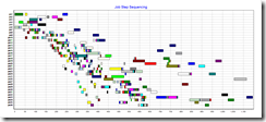
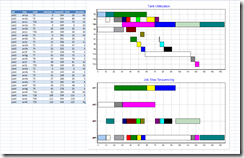
image

Large scale example:

tankchart1 tankchart2

Tuesday, July 20, 2010

Tough little MIP's

These are two instances (related to http://yetanothermathprogrammingconsultant.blogspot.com/2010/07/multiple-length-cutting-stock-problem.html) of very small MIP models that are very tough to solve to optimality. Size is very small: 26 rows and 73 columns. The first data set solves slowly, but the second one is really tough even for the best MIP solvers (at least with default settings).

Usually models of this size solve very quickly, but with MIP’s one should always be prepared for surprises.

Workaround: just stop after a little while: the obj is most likely optimal just not proven optimal. This behavior is not unusual: the mip solvers have good heuristics so they actually find the (near) optimal solution very quickly. But proving optimality by working on the best bound is not that easy and turns out to be very expensive. A second approach would be to use the alternative formulation mentioned in http://yetanothermathprogrammingconsultant.blogspot.com/2010/07/multiple-length-cutting-stock-problem.html.

To prove optimality it makes sense to use an option like MipEmphasis (Cplex) or MipFocus (Gurobi) to move the best bound. Dataset 1 then solves quite quickly but dataset 2 is still terrible.

Point two filenames to the same file?

In Windows there are many ways to describe the same file: UNC, old 8.3 notation, relative, absolute. Unfortunately it is not trivial to detect whether two filenames are pointing to the same file. Here is some code that does this: http://blogs.msdn.com/b/vbteam/archive/2008/09/22/to-compare-two-filenames-lucian-wischik.aspx.

(Under Unix I guess one would use the inode to check this)

Monday, July 12, 2010

Max Availability in Cutting Stock Model

In http://yetanothermathprogrammingconsultant.blogspot.com/2010/07/multiple-length-cutting-stock-problem.html an extension of the standard cutting stock model is discussed. A question was posed if it would be difficult to add some availability restriction to this model. I.e. example data can look like:
image
This can be implemented as follows. Our notation is again:
imageThen the master problem in the column generation approach can look like:
imagewhere we have the following constants:
imageThe subproblem can be formulated as:
image The initialization of the algorithm needs a little bit more sophistication than I had before, to make sure a feasible initial solution is created. Alternatively it may be more convenient to make the master elastic with respect to the availability constraint, so that it is easier to construct a feasible solution.

An example solution can look like:
 

Sunday, July 4, 2010

GAMS: display

While playing with my old column generation example http://www.amsterdamoptimization.com/pdf/colgen.pdf I wanted to change the display of of the patterns a little bit:

----    181 PARAMETER pat  pattern usage

                 p1         p15         p18         p21         p25         p26         p28         p31         p34

width1       12.000                               2.000                               1.000
width2                    1.000       3.000       2.000                   1.000       1.000
width3                                            2.000       2.000       3.000                               1.000
width4                                3.000
width5                                                                                            2.000
width6                                                        1.000       1.000                   4.000       5.000
width7                                                                                3.000
width9                    3.000
width10                                                                                           1.000       1.000
width13                                                       2.000                                           1.000
Count         4.000      27.000      49.000      61.000       1.000     222.000     479.000      61.000       3.000

      +         p36         p37         p38         p39         p40         p42         p43         p44         p45

width1                                            1.000                   4.000
width2                                2.000                   1.000                                           4.000
width3        1.000       2.000       1.000       1.000                   1.000       2.000       2.000
width4                                            3.000                               1.000
width6        1.000       5.000       1.000       2.000       4.000                               1.000
width7        1.000                                                                   1.000                   1.000
width8                                1.000
width9                                                                                            1.000
width10                                                                               2.000                   1.000
width11                               2.000                   3.000       3.000                   1.000
width12                   1.000
width13       2.000
Count       191.000     101.000     103.000       1.000      79.000       1.000       1.000     347.000      20.000

      +       Total

width1      654.000
width2     1362.000
width3     1987.000
width4      151.000
width5      122.000
width6     1946.000
width7     1649.000
width8      103.000
width9      428.000
width10      86.000
width11     793.000
width12     101.000
width13     387.000
Count      1751.000

Now I wanted to drop the zero’s after the decimal point, so I did:

option pat:0;
display pat;

This gave as result:

----    183 PARAMETER pat  pattern usage

                 p1         p15         p18         p21         p25         p26         p28         p31         p34

width1           12                                   2                        ***********1
width2                        1           3           2                       1           1
width3                                                2           2           3                                   1
width4                                    3
width5                                                                                                2
width6                                                            1           1                       4           5
width7                                                                                    3
width9                        3
width10                                                                                               1           1
width13                                                           2                                               1
Count             4          27          49          61           1         222         479          61           3

      +         p36         p37         p38         p39         p40         p42         p43         p44         p45

width1                                                1                       4
width2                                    2                       1                                               4
width3            1           2           1           1                       1           2           2
width4                                                3                                   1
width6            1           5           1           2           4                                   1
width7            1                                                                       1                       1
width8                                    1
width9                                                                                                1
width10                                                                                   2                       1
width11                                   2                       3           3                       1
width12                       1
width13           2
Count           191         101         103           1          79           1           1         347          20

      +       Total

width1          654
width2         1362
width3         1987
width4          151
width5          122
width6         1946
width7         1649
width8          103
width9          428
width10          86
width11         793
width12         101
width13         387
Count          1751

It is not clear what the stars are doing there. May be some debugging output left in the code.

Multiple length cutting stock problem

I received some test data to run against a cutting stock model (see http://yetanothermathprogrammingconsultant.blogspot.com/2009/09/vstosolver-foundation.html). The data approximately looks like:
image This cannot be solved using the standard model mentioned here and in http://www.amsterdamoptimization.com/pdf/colgen.pdf. The standard model assumes there is just one raw material length, and we have here a number of different lengths in stock. Note that we assume that stock availability is not a limiting factor. The question was: can we adapt the column generation approach to handle this.
The first document I found with google was this: http://www.aimms.com/aimms/download/manuals/aimms3om_cuttingstock.pdf. At first reading this did not look very promising for different reasons. First they use as objective in the multiple length version: minimize the cost of each stock length. I don’t have this data available, and we are aiming to minimize waste.  Note that in the standard cutting stock problem we can simply use the number of rolls of raw material as proxy to find the minimum waste. In this case this is not a good objective and we really need to model the wasted material explicitly.
A second problem was the simple way they dealt with the multiple lengths in the sub problem. They just run the subproblem several times:
image
In our case we have a somewhat large set of stock lengths, so that is not attractive. It was argued one could stop as soon as a good candidate was found. (Note: There is some confusion about what the sub and the master is as they use the term submodel for what usually is called the master problem.)
I believe there is a more elegant way to do this: let the pattern generation model (this is usually called the subproblem) find a candidate pattern and a candidate raw material length directly. A similar approach is written up here.
So with the notation:
image
we have:
image
and we can form a master problem as follows:
image
Note that I used an equality constraint here. That is to make sure we don’t produce more products with zero waste than needed. The subproblem can now look like:
image
Here lambda are the duals of the master problem. So the subproblem both finds a new pattern y(i) and which stock length k is to be used for this pattern. This actually solved the problem quickly (approx 10 seconds). A further improvement was added by preprocessing the data. If a demand length is equal to a stock length, we can immediately choose that stock length, and remove this demand from the model. If the problem is larger, it may be wise to add a tolerance, i.e. if a demanded length is within say 5% of a stock length, use that stock length.
It is interesting to see that the column generation algorithm actually is not that sensitive to the preprocessing step:
image
We stop a little bit earlier with preprocessing, but the expected better performance is not uniformly over the whole run. It is noted I used a simple minded assignment for the initial solution. Probably a simple bin-packing heuristic to find an initial solution can help to start the column generation algorithm with a better objective.
An alternative formulation would be: use inequality constraint in the master together with a cost coefficient of c(p)=L(k(p)). The subproblem needs to be updated slightly: drop U from the objective. This formulation gave similar results.

The solution looks like: