The different coloring of decision variables and parameters can help understanding the equations. In this case x is a parameter (this is typical when we implement estimation problems in GAMS: the statistical variables become parameters, while coefficients in the statistical model – here β and µ – are decision variables in the optimization model).
I am a full-time consultant and provide services related to the design, implementation and deployment of mathematical programming, optimization and data-science applications. I also teach courses and workshops. Usually I cannot blog about projects I am doing, but there are many technical notes I'd like to share. Not in the least so I have an easy way to search and find them again myself. You can reach me at erwin@amsterdamoptimization.com.
Friday, December 19, 2014
Convert GAMS to LaTeX
Monday, December 15, 2014
No multiple objectives?
In http://fdahms.com/2014/12/05/objective_functions/ it is argued that we should not fall in the “multi objective trap”. In my experience many practical models have some multi-objective structure. Some examples of models I have been working on are:
- Return vs risk. e.g. portfolio models
- Scheduling: minimize number of late (I should say tardy) jobs vs sum of of tardiness. If only number of late jobs is considered, it does not matter how late a late job is. In practice a job being late a little bit is better. On the other hand the minimizing the sum may deliver a ton of jobs being a little late. Combining these objectives can help.
- Scheduling: adding an extra objective that minimizes the difference between an existing schedule and the new schedule can help preventing wild changes in schedules without having a clear benefit (persistency).
- Cost vs Customer Service Level. If we can improve the CSL when it costs very little we may want to exploit this. On the other hand if a small decrease in CSL delivers a ton of profit then that is also worth considering.
- Tank design: cost vs fire power vs weight.
- Supply chain: cost vs robustness. E.g. keep extra suppliers although reducing the number of suppliers may reduce cost.
- In a typical Cost – Benefit Analysis we also have to consider several criteria.
- Soft and elastic constraints will give rise to extra objectives.
- Etc, etc,
In my view many if not most interesting practical problems have conflicting goals and objectives. To make the client aware of this is an important role of a modeler. Even if we solve this as a single objective model using weights and penalties, the modeler needs to be aware and communicate the multi-objective nature and trade-offs of the underlying model.
Sunday, December 14, 2014
Modeling number of machine start-ups
I came a across an extension of a well-known problem: counting the number of start-ups of a machine.
In the power generation models we often see constraints related to the number of start-ups of a generator: because of wear and tear we may like to minimize or restrict the number of times a generator is turned on. In the picture below the x(i) vector is the state of a generator (on or off) and the s(i) vector indicates when a startup occurs (i is time period). Both x and s are binary variables.
If we are minimizing the number of startups or have an upper bound, this can be easily modeled with a single inequality:
Here s(i) is forced to be one if there is a start-up, otherwise it is unrestricted. I.e. as long as the bound U is not binding we may have a few elements in s being 1 while there is no real start-up there. This is a structure we often see in models.
A lower bound on the number of startups is somewhat unusual, but lets see what happens. If we have a lower bound on the number of start-ups we need to be more precise and force s(i)=0 if there is no start-up. This can be modeled as:

The state in period zero is assumed to be known. This matters if we have x(i)=1 in the first period. This is only counted as a startup in case the initial state is 0. In GAMS we can model this compactly as:
The trick with the initial state resembles how we can deal with iniitial inventory in a supply chain model. See: http://yetanothermathprogrammingconsultant.blogspot.com/2014/10/handling-of-inventory.html.
Saturday, December 13, 2014
Gurobi 6 Distributed vs Concurrent MIP
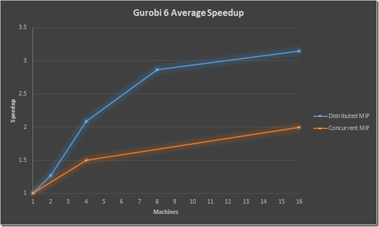
The new Gurobi 6 has quite an attractive offering for running distributed MIPs. Here is a summary for their results (MIPLIB models taking more than 100s).
The concurrent MIP method is just running the same model on different machines with a different random number seed. This changes the solution path sufficiently to actually form a feasible parallel approach. The solution time is the time of the winner. This method always amazes me, but also makes me feel somewhat uncomfortable (the scary question is: if this scheme works does the MIP solver really know what it is doing? – My answer often depends on whether the last MIP I tried was solved ok.). See e.g.: http://coral.ie.lehigh.edu/~jeff/mip-2008/talks/danna.pdf
The distributed MIP is really a distributed MIP where each machine works on parts of the tree. Happy to see this actually works a bit better. Before you buy a ton of machines note that performance starts to tail off after using more than 8 machines. Some numbers showed that a bunch of smaller machines may show better performance than a huge multi-core machine (these SMP machine suffer from memory contention, probably exacerbated by MIP solvers jumping around in memory i.e. suffering from limited locality which hampers exploiting even large caches). Typically several small machines is cheaper than one big one.
Note that every machine in the above picture is actually equipped with a 4 core CPU, so we already have significant parallelism on each machine.
Some other new features:
- Some support for piecewise linear functions. In the objective only and convex only so for a limited class of models for now. Non-convex functions are translated into a MIP formulation.
- General improvements in performance
- Enhancements in lazy constraints
Thursday, December 11, 2014
Optimization in R
Some interesting notes:
From: http://user2014.stat.ucla.edu/files/tutorial_Nash_slides.pdf:
My opinion: I think GAMS and R non-linear optimization really targets different audiences and different model types (R: smaller models with emphasis on parameter estimation and zero or few constraints; GAMS: large, sparse and more complex models with many constraints). Matlab and R may be seen a little bit more as direct “competitors” with respect to the type models they typically solve.
Amazon seems to confirm people are using R to do optimization:
Tuesday, December 2, 2014
Big Iron vs my laptop
- Model runs runs fast on both. This is what I like most. In this case of course running locally is often easier: the big iron does not really help. This is a large class of problems (helped by good solvers and lots of modeling experience).
- Model runs slow on laptop and slow on big machine. The expensive hardware does not help here. This also happens quite frequently. Solution: rework the problem (e.g. reformulations, aiming for good solutions, heuristics etc). Hopefully moving the problem to category 1.
- Model runs slow on my laptop but fast on the big machine. This actually does not happen too often. The number of models that falls in this category is surprisingly small.
- Model runs fast on my laptop and slow on the big machine. This should not happen, but it actually does. Often my optimization problems run surprisingly slow on expensive hardware. Some reasons: the cluster has expensive hardware from a few years ago (my laptop is new every year), there may be latencies in starting jobs on a cluster, it may have been too expensive to get the best solvers on the big machines (I think IBM counts VPUs which can add up) or much parallelization does not pay off. Big caches may help less than expected for some sparse data structures used in modeling systems and solvers. Another reason is often; not enough memory. Running n parallel jobs may require n times the memory. I have seen clients being somewhat underwhelmed or even disappointed by performance on what was sold as very expensive (and fast) hardware.
Wednesday, November 26, 2014
Example of use of Unit Loss Function
In a previous post I showed how to write and solve a unit loss function G(k). Here I show how to use it.
Here I solve some (s,Q) inventory models. These models have a variable Q: order quantity. It is sometimes argued to use the EOQ order quantity for this. EOQ stands for Economic Order Quantity. In the model I try to see how much difference it makes when we use this EOQ or just solve for Q in the (s,Q) models directly.
The results are:
| ---- 155 PARAMETER results EOQ Qendog Qeoq EOQ .Q 5200.000 |
We can see for two inventory models (Cost per Stockout Event – CSOE and Cost per Item Short – CIS) the differences in Q and s are significant. However the effect on total cost and relevant cost is more limited: things are pretty flat out there.
In practice formulas based on the first order conditions are used to solve these inventory models. However I think there is a case to be made to look at the original cost functions and optimize these directly. This relates more to the original problem and also we may be a little bit more flexible if we want to add a few more wrinkles. In some cases there are closed solutions, e.g. the well known EOQ formula is:
In the model below again we use the original cost function and minimize that for Q. Note that for other cases it may not be that easy to find closed solutions.
| $ontext |
Thursday, November 20, 2014
Unit Loss Function
A standard normal unit loss function can be described as:
where f(x) is the standard normal density function and F(x) is the standard normal CDF. See: http://planetmath.org/unitnormallossfunction.
Often we want to solve UNL(x)=c for x.
GAMS Version
| $ontext |
This solves with CONOPT very quickly, we get:
Note: the GAMS math expressions can be inspected with a new tool. This is a nice test example:
Wolfram Alpha
The input is easy:
The output is unfortunately:
Mathematica
The above approach is not really suited for Mathematica. This looks better:
R
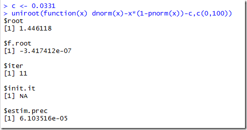
Super easy input, due to predefined functions for normal pdf and cdf. We give an interval of [0,100] to search:
Excel
Its root finder is called Goal Seek.
It is a little bit sloppy by default. We can make Goal Seek more precise by multiplying the UNC-c cell by a 1000:
Note: the tolerance can also be set in the Excel options (under formulas, Maximum Change). Looks like Excel is using an absolute tolerance on Δx and Δf (i.e. it could stop prematurely if the algorithm chooses a very small Δx).
Python
Quite nice:


