Strange objective

In [1], a question was posted how to use the $\mathit{sign}()$ function in the SCIP solver. The problem to solve is

argmax(w) sum(sign(Aw) == sign(b)) 

This is a strange objective. Basically: find $w$, with $v=Aw$ such that we maximize the number of  $v_i$ having the same sign as $b_i$. I have never seen such an objective.

As $A$ and $b$ are constants, we can precompute $$\beta_i = \mathrm{sign}(b_i)$$ This simplifies the situation a little bit (but I will not need it below).

A different way to say "$v_i$ and $b_i$ have the same sign" is to state: $$v_i b_i > 0$$ I assumed here $b_i \ne 0$. Similarly, the constraint $v_i b_i < 0$ means: "$v_i$ and $b_i$ have the opposite sign."

If we introduce binary variables: $$\delta_i = \begin{cases} 1 & \text{if $ v_i b_i > 0$}\\ 0 & \text{otherwise}\end{cases}$$ a model can look like: $$\begin{align} \max & \sum_i \delta_i \\ &\delta_i =1 \Rightarrow \sum_j a_{i,j} b_i w_j > 0 \\ & \delta_i \in \{0,1\}\end{align}$$ The implication can be implemented using indicator constraints, so we have now a linear MIP model.

Notes:

• I replaced the $\gt$ constraint by $\sum_j a_{i,j} b_i w_j \ge 0.001$ 
• If the $b_i$ are very small or very large we can replace them by $\beta_i$, i.e. $\sum_j a_{i,j} \beta_i w_j \gt 0$
• The case where some $b_i=0$ is somewhat ignored here. In this model, we assume $\delta_i=0$ for this special case. 
• We can add explicit support for  $b_i=0$ by:   $$\begin{align} \max & \sum_i \delta_i \\ &\delta_i =1 \Rightarrow \sum_j a_{i,j} b_i w_j > 0 && \forall i | b_i\ne 0 \\ & \delta_i =1 \Rightarrow \sum_j a_{i,j} w_j = 0 && \forall i | b_i = 0  \\ & \delta_i \in \{0,1\}\end{align}$$
• We could model this with binary variables or SOS1 variables. Binary variables require big-M values. It is not always easy to find good values for them. The advantage of indicator constraints is that they allow an intuitive formulation of the problem while not using big-M values. 
• Many high-end solvers (Cplex, Gurobi, Xpress, SCIP) support indicator constraints. Modeling systems like AMPL also support them.

Test with small data set

Let's do a test with a small random data set.

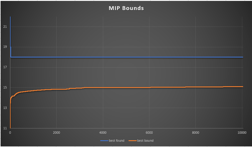
----     17 PARAMETER a  random matrix

             j1          j2          j3          j4          j5

i1       -0.657       0.687       0.101      -0.398      -0.416
i2       -0.552      -0.300       0.713      -0.866 4.213380E-4
i3        0.996       0.157       0.982       0.525      -0.739
i4        0.279      -0.681      -0.500       0.338      -0.129
i5       -0.281      -0.297      -0.737      -0.700       0.178
i6        0.662      -0.538       0.331       0.552      -0.393
i7       -0.779       0.005      -0.680       0.745      -0.470
i8       -0.428       0.188       0.445       0.256      -0.072
i9       -0.173      -0.765      -0.372      -0.907      -0.323
i10      -0.636       0.291       0.121       0.540      -0.404
i11       0.322       0.512       0.255      -0.432      -0.827
i12      -0.795       0.283       0.091      -0.937       0.585
i13      -0.854      -0.649       0.051       0.500      -0.644
i14      -0.932       0.170       0.242      -0.221      -0.283
i15      -0.514      -0.507      -0.739       0.867      -0.240
i16       0.567      -0.400      -0.749       0.498      -0.862
i17      -0.596      -0.990      -0.461 -2.97050E-4      -0.697
i18      -0.652      -0.339      -0.366      -0.356       0.928
i19       0.987      -0.260      -0.254       0.544      -0.207
i20       0.826      -0.761       0.471      -0.889       0.153
i21      -0.897      -0.988      -0.198       0.040       0.258
i22      -0.549      -0.208      -0.448      -0.695       0.873
i23      -0.155      -0.731      -0.228      -0.251      -0.463
i24       0.897      -0.622      -0.405      -0.851      -0.197
i25      -0.797      -0.232      -0.352      -0.616      -0.775


----     17 PARAMETER b  random rhs

i1   0.193,    i2   0.023,    i3  -0.910,    i4   0.566,    i5   0.891,    i6   0.193,    i7   0.215,    i8  -0.275
i9   0.188,    i10  0.360,    i11  0.013,    i12 -0.681,    i13  0.314,    i14  0.048,    i15 -0.751,    i16  0.973
i17 -0.544,    i18  0.351,    i19  0.554,    i20  0.865,    i21 -0.598,    i22 -0.406,    i23 -0.606,    i24 -0.507
i25  0.293


----     17 PARAMETER beta  sign of b

i1   1.000,    i2   1.000,    i3  -1.000,    i4   1.000,    i5   1.000,    i6   1.000,    i7   1.000,    i8  -1.000
i9   1.000,    i10  1.000,    i11  1.000,    i12 -1.000,    i13  1.000,    i14  1.000,    i15 -1.000,    i16  1.000
i17 -1.000,    i18  1.000,    i19  1.000,    i20  1.000,    i21 -1.000,    i22 -1.000,    i23 -1.000,    i24 -1.000
i25  1.000


----     53 VARIABLE w.L  

j1 -0.285,    j2 -0.713,    j3 -0.261,    j4 -0.181,    j5 -0.630


----     53 PARAMETER v  sum(j, a(i,j)*w(j))

i1   0.005,    i2   0.342,    i3  -0.282,    i4   0.556,    i5   0.498,    i6   0.256,    i7   0.557,    i8  -0.129
i9   1.059,    i10  0.099,    i11  0.076,    i12 -0.197,    i13  1.008,    i14  0.299,    i15  0.695,    i16  0.771
i17  1.435,    i18  0.003,    i19  0.002,    i20  0.249,    i21  0.843,    i22 -0.002,    i23  0.962,    i24  0.571
i25  1.084


----     53 VARIABLE delta.L  

i1  1.000,    i2  1.000,    i3  1.000,    i4  1.000,    i5  1.000,    i6  1.000,    i7  1.000,    i8  1.000
i9  1.000,    i10 1.000,    i11 1.000,    i12 1.000,    i13 1.000,    i14 1.000,    i16 1.000,    i18 1.000
i19 1.000,    i20 1.000,    i22 1.000,    i25 1.000


----     53 VARIABLE z.L                   =       20.000  objective variable

This means, for this 25 row problem we can find $w$'s such that 20 rows yield the same sign as $b_i$.

References

1. SCIP What is the function for sign?, https://stackoverflow.com/questions/53030430/scip-what-is-the-function-for-sign

Gurobi 8.1

Quite some improvements in MIQP performance. Of course the smaller improvements in other model types also help: over time these things add up to substantial performance gains.

Announcement

Gurobi is pleased to announce the release of Gurobi Version 8.1. This latest version improves the overall performance of Gurobi Optimizer, and adds enhancements to Gurobi Instant Cloud, including support for Microsoft Azure® and for the latest Amazon Web Services® machines, and more.

Version 8.1 demonstrates our commitment to delivering the new features our users request, and includes:

Performance Improvements

Gurobi Optimizer v8.1 continues to push the envelope of solver speed and performance. The overall v8.1 performance improvements versus v8.0 include:

MIQP 

• More than a factor of 2.8x faster overall.
• More than a factor of 6x faster on difficult models that take more than 100 seconds to solve.

MIQCP

• 38% faster overall.
• 92% faster on difficult models that take more than 100 seconds to solve.

LP

• 2.9% faster overall in default settings.
• 6.5% faster on difficult models that take more than 100 seconds to solve.

LP barrier

• 4.4% faster overall.
• 11% faster on difficult models that take more than 100 seconds to solve.

LP dual simplex

• 4.2% faster overall.
• 10.5% faster on difficult models that take more than 100 seconds to solve.

---

Enhancements

• Gurobi Instant Cloud now supports Microsoft Azure®: Instant Cloud users can now use Microsoft Azure, in several regions.
• Gurobi Instant Cloud adds faster and more powerful machines on Amazon EC2®: The new version supports c5, r5 and z1 instance types.
• New Q matrix linearization for MIQP and MIQCP models: We added a new Q matrix linearization approach in presolve. This new option can be chosen by setting parameter PreQLinearize to the new value of 2.
• Improved Mac Installation Package: Users no longer need to install Xcode to perform the installation.
• Support for Python 3.7: We have added support for Python 3.7 on Windows, Linux and Mac platforms.
• A callback function for multi-objective optimization: We now let users terminate optimization for individual objectives for multi-objective MIP models.

To learn more about all of the new features and improvements, visit What's New in Gurobi 8.1.

The Muffin Problem

We are asked to split $m=5$ muffins between $s=3$ students, such that each student gets in total $$\frac{m}{s} = \frac{5}{3}$$ worth of muffins [1]. From [2] we see two possible ways of doing this:

Allocation 1 (from [2])

Allocation 2 (from [2])

(I believe Proc means Procedure). The problem is to find a way to divide the muffins such that the smallest piece is maximized.

There is a nice and simple MIP formulation for this. Let's define $x_{i,j} \in [0,1]$ as the fraction of muffin $i$ assigned to student $j$. Also we need: $$\delta_{i,j} = \begin{cases} 1 & \text{if $x_{i,j} \gt 0$} \\ 0 & \text{if $x_{i,j}=0$}\end{cases}$$ Then we can write:

Muffin Problem

$$\begin{align}\max\> & \color{DarkRed} z \\ & \sum_i \color{DarkRed} x_{i,j} = \color{DarkBlue} {\frac{m}{s}} && \forall j\\ & \sum_j \color{DarkRed} x_{i,j} = 1  && \forall i\\ & \color{DarkRed} \delta_{i,j} = 0 \Rightarrow \color{DarkRed} x_{i,j} = 0 \\ & \color{DarkRed} \delta_{i,j} = 1 \Rightarrow \color{DarkRed} z \le \color{DarkRed} x_{i,j} \\ & 0 \le \color{DarkRed} x_{i,j} \le 1\\ & \color{DarkRed} \delta_{i,j} \in \{0,1\}\end{align}$$

The objective takes care of $x_{i,j}=0 \Rightarrow \delta_{i,j}=0$. Some MIP solvers allow us to use the implications directly (as so-called indicator constraints). For others we need to reformulate. It is not difficult to rewrite them as inequalities:

Implication	Inequality
$$\color{DarkRed} \delta_{i,j} = 0 \Rightarrow \color{DarkRed} x_{i,j} = 0$$	$$\color{DarkRed} x_{i,j} \le \color{DarkRed} \delta_{i,j}$$
$$\color{DarkRed} \delta_{i,j} = 1 \Rightarrow \color{DarkRed} z \le \color{DarkRed} x_{i,j}$$	$$\color{DarkRed} z \le \color{DarkRed} x_{i,j}+ (1-\color{DarkRed} \delta_{i,j})$$

This is similar to what is proposed in [1] (they use $y_{i,j} = 1-\delta_{i,j}$) and somewhat simpler than the approach used in [3].

The results are:

----     26 VARIABLE x.L  fraction of muffin assigned to student

           student1    student2    student3

muffin1       0.500                   0.500
muffin2       0.583       0.417
muffin3                   0.417       0.583
muffin4       0.583       0.417
muffin5                   0.417       0.583


----     26 VARIABLE d.L  indicator for nonzero x

           student1    student2    student3

muffin1       1.000                   1.000
muffin2       1.000       1.000
muffin3                   1.000       1.000
muffin4       1.000       1.000
muffin5                   1.000       1.000


----     26 VARIABLE z.L                   =        0.417  smallest nonzero x

If student1 arrives early and confiscates muffin1, we can fix $x_{\text{muffin1},\text{student1}}=1$. With this we can reproduce the first solution:

----     28 VARIABLE x.L  fraction of muffin assigned to student

           student1    student2    student3

muffin1       1.000
muffin2                   1.000
muffin3       0.333       0.667
muffin4                               1.000
muffin5       0.333                   0.667


----     28 VARIABLE z.L                   =        0.333  smallest nonzero x

A solution for 7 muffins and 5 students can look like:

----     26 VARIABLE x.L  fraction of muffin assigned to student

           student1    student2    student3    student4    student5

muffin1       0.667       0.333
muffin2       0.333                   0.667
muffin3       0.400       0.600
muffin4                               0.333       0.333       0.333
muffin5                   0.467                               0.533
muffin6                                           0.467       0.533
muffin7                               0.400       0.600


----     26 VARIABLE z.L                   =        0.333  smallest nonzero x

Not all problems are super easy to solve to proven optimality. E.g. with 11 muffins and 9 students, I had to spend several minutes. As usual the solver quickly found the optimal solution, but proving optimality was not so quick. There is lots of symmetry in the model. That may be something to exploit.

References

1. Guangiqi Cui, John Dickerson, Naveen Durvasula, William Gasarch, Erik Metz, Jacob Prinz, Naveen Raman, Daniel Smolyak, Sung Hyun Yoo, The Muffin Problem, 13 Mar 2018, https://arxiv.org/pdf/1709.02452.pdf
2. https://www.cs.umd.edu/~gasarch/muffintalk.pdf
3. https://math.stackexchange.com/questions/2958179/how-to-prove-that-1-3-is-the-optimal-solution-for-the-muffin-problem-with-5-stud
4. NRC (Dutch newspaper), https://www.nrc.nl/nieuws/2018/09/14/hoe-vijf-muffins-tot-een-diep-wiskundig-vraagstuk-leidden-a1616534

A pure fixed charge transportation problem

The standard transportation problem is an example of an easy linear programming problem:

Transportation Problem
$$\begin{align}\min & \sum_{i,j} \color{DarkBlue} c_{i,j} \color{DarkRed} x_{i,j}\\ & \sum_j \color{DarkRed} x_{i,j} = \color{DarkBlue} {\mathit{supply}}_i\\ & \sum_i \color{DarkRed} x_{i,j} = \color{DarkBlue} {\mathit{demand}}_j \\ & \color{DarkRed} x_{i,j} \ge 0\end{align}$$

We can solve very large instances very quickly. The fixed charge transportation problem is much more difficult:

Fixed Charge Transportation Problem

$$\begin{align}\min & \sum_{i,j} \color{DarkBlue} c_{i,j} \color{DarkRed} x_{i,j} + \color{DarkBlue} d_{i,j} \color{DarkRed} y_{i,j}\\ & \sum_j \color{DarkRed} x_{i,j} = \color{DarkBlue} {\mathit{supply}}_i\\ & \sum_i \color{DarkRed} x_{i,j} = \color{DarkBlue}{\mathit{demand}}_j \\ & 0 \le \color{DarkRed} x_{i,j} \le \color{DarkBlue} M \color{DarkRed} y_{i,j}\\ & \color{DarkRed} y_{i,j} \in \{0,1\}\end{align}$$

Here we have an additional cost $d_{i,j}$ if link $x_{i,j}$ is used (i.e. if $x_{i,j}\gt 0$).  The binary variable $y_{i,j}$ indicates if link $i \rightarrow j$ is used. I.e. we want: $$y_{i,j} = 0 \Rightarrow x_{i,j}=0$$ The constraint $x_{i,j} \le M y_{i,j}$ is a big-M formulation for this. Notice that we do not need to worry about $x_{i,j}=0 \Rightarrow y_{i,j}=0$: this will be taken care of automatically (because of the objective function). In practice we can do $$\begin{align} & x_{i,j} \le M_{i,j} y_{i,j}\\ & M_{i,j} = \min \{ \mathit{supply}_i,  \mathit{demand}_j \}\end{align}$$ This gives some reasonable values for $M_{i,j}$. A problem with only fixed charge costs (i.e. $c_{i,j}=0$) is sometimes called a pure fixed charge transportation problem. If we just want to minimize the number of links that are being used we can set $c_{i,j}=0$ and $d_{i,j}=1$. These models can be incredibly difficult to solve to proven optimality.

Here we try to solve a very small problem with 10 source nodes and 10 destination nodes. I used random values for the supply and demand:

----     20 PARAMETER supply  

src1  0.041,    src2  0.203,    src3  0.132,    src4  0.072,    src5  0.070,    src6  0.054,    src7  0.084
src8  0.206,    src9  0.016,    src10 0.120


----     20 PARAMETER demand  

dest1  0.178,    dest2  0.103,    dest3  0.177,    dest4  0.136,    dest5  0.023,    dest6  0.114,    dest7  0.028
dest8  0.045,    dest9  0.119,    dest10 0.078

The objective is $\min \sum_{i,j} y_{i,j}$, i.e. we minimize the number of open links. This means we have just 100 binary variables. After setting a time limit of 9999 seconds I see:

. . .  5938307 5589691       15.7946    12       18.0000       15.0950 1.71e+08   16.14%  5946634 5596825       15.1040    25       18.0000       15.0950 1.72e+08   16.14%  5959435 5611506       15.1737    19       18.0000       15.0950 1.72e+08   16.14% Elapsed time = 9977.59 sec. (3226694.74 ticks, tree = 38155.78 MB, solutions = 3) Nodefile size = 36108.12 MB (23960.92 MB after compression)  5965049 5616397       16.0000    19       18.0000       15.0950 1.72e+08   16.14% Cover cuts applied:  264 Flow cuts applied:  5 Mixed integer rounding cuts applied:  331 Zero-half cuts applied:  4 Multi commodity flow cuts applied:  4 Root node processing (before b&c):   Real time             =    0.88 sec. (41.53 ticks) Parallel b&c, 8 threads:   Real time             = 10021.94 sec. (3248441.83 ticks)   Sync time (average)   = 5484.02 sec.   Wait time (average)   =    0.11 sec.                           ------------ Total (root+branch&cut) = 10022.81 sec. (3248483.36 ticks) MIP status(107): time limit exceeded Cplex Time: 10023.03sec (det. 3248483.36 ticks)

Ouch.. If you would have asked before, I certainly would have predicted somewhat better performance.

MIP bounds don't change anymore

The best objective value of 18 was found after 25 seconds.  We might as well have stopped at that point...

Most likely 18 is the optimal objective, but we have not proven that. The best solution looks like:

Best found solution

Just your average Excel formula

Source:
Ira Iosebashvili, Wall Street Journal, The First Rule of Microsoft Excel -- Don't Tell Anyone You're Good at it, Oct. 5, 2018
https://www.wsj.com/articles/the-first-rule-of-microsoft-exceldont-tell-anyone-youre-good-at-it-1538754380

Scheduling and three sided football

Design a tournament schedule

In [1] a question is posed how to design a schedule for a sequence games:

• There are 9 teams,
• we have 4 rounds of 3 matches,
• each match consists of 3 teams,
• a team plays with another team exactly once in the same match.

This problem is related to the social golfer problem [2,3]. Not many games have three teams but there is something called three sided football [4].

Three sided football field [4]

Integer Quadratically Constrained Model

To find a feasible schedule we use the following sets: $$\begin{align} & t \in \{A,\dots,I\} && \text{9 teams} \\ & r \in \{\mathit{round}_1,\dots,\mathit{round}_4\} && \text{4 rounds}\\ & m \in \{\mathit{match}_1,\dots,\mathit{match}_3\} && \text{3 matches per round} \end{align}$$ We introduce binary variables $$x_{r,m,t} = \begin{cases} 1 & \text{if team $t$ plays in match $m$ in round $r$} \\ 0 & \text{otherwise}\end{cases}$$
A high-level model can look like:

MIQCP feasibility model
$$\sum_m x_{r,m,t} = 1 \>\>\forall r,t$$	Each team plays exactly once in each round
$$\sum_t x_{r,m,t} = 3 \>\>\forall r,m$$	Each match consists of three teams
$$\sum_{r,m} x_{r,m,t} x_{r,m,t'} = 1 \>\>\forall t\lt t'$$	Teams $t$ and $t'$ play exactly once in the same match. This is a non-convex, quadratic constraint.

There is no objective: we are only looking for a feasible solution. The last equation is the most complicated one. We have $x_{r,m,t} x_{r,m,t'}=1$ if teams $(t,t')$  are in the same match $(r,m)$. Because of symmetry in the product $x_{r,m,t} x_{r,m,t'}$ , we only need to check teams $t\lt t'$. This saves us a few quadratic constraints.

This model can be solved with a constraint solver or a global (non-convex) MIQCP (Mixed Integer Quadratically Constrained Programming) solver. Of course, with a MIQCP solver we need to add a dummy objective. Global solvers, like Baron, Couenne or Antigone, can solve this easily. The results can look like:

Solution

We have marked the cases where $x_{r,m,t}=1$. We can check that:

• Every row has three entries (a match has three teams)
• Every column has four entries: one in each round (a team plays once in each round)
• Two teams play in the same match exactly once (e.g. A and B meet in round 1 only)

It is noted that there are many feasible solutions.

Making the problem convex, linear

If we want to solve with a convex MIQCP solver (like Cplex or Gurobi) we can replace the quadratic constraint by: $$\sum_{r,m} x_{r,m,t} x_{r,m,t'} \le 1 \>\>\forall t\lt t'$$

Finally, if we want, we can linearize the quadratic constraint. That would allow us to solve this problem with a straight linear MIP solver. We can write: $$\begin{align} & y_{r,m,t,t'} \ge x_{r,m,t} + x_{r,m,t'} - 1 && \forall r,m,t\lt t'\\ & \sum_{r,m} y_{r,m,t,t'} \le 1 && \forall t\lt t'\\ &   y_{r,m,t,t'} \in [0, 1]\end{align}$$ Again, we need to do this only for $t\lt t'$. The MIP model performs better than the quadratic versions if the problems become a bit larger. It is not unusual that linarized models, solved as a MIP, perform better than using a quadratic solver against the original model, even if we have to add a significant number of variables and equations in the process.

There is lots of symmetry in this problem and there are quite a few papers around, mainly from a constraint programming view, that try to deal with this.

Fixing

For larger problems there are a few tricks we can apply. For example, we can fix the first two rounds, and let the model only worry about the subsequent rounds. In addition we can fix the first $m$ teams in all rounds. The idea is to make the remaining problem smaller so that the solver has an easier job. Fixing also reduces symmetry. With this I could solve very quickly the following instances [5] (I used the MIP formulation):

5 rounds, 4 matches, 16 teams (first 2 rounds, first 4 teams fixed)

6 rounds, 5 matches, 25 teams (first 2 rounds, first 5 teams fixed)

The dark areas were fixed and the light area was solved by the MIP solver.

Conclusion

With two simple tricks:

• linearization of the quadratic constraint 
• fixing a significant part of the problem

we can solve reasonable sized schedule design problems with a good MIP solver quickly. 

References

1. PHP - Evenly Distribute Teams Into Arrays So That No Combination Repeats, https://stackoverflow.com/questions/52600546/php-evenly-distribute-teams-into-arrays-so-that-no-combination-repeats
2. Markus Triska and Nysret Musliu, An Improved SAT Formulation for the Social Golfer Problem, Annals of Operations Research Vol. 194(1) (2012), pp. 427-438
3. Nicolas Barnier, Pascal Brisset. Solving the Kirkman’s schoolgirl problem in a few seconds. CP 2002, 8th International Conference on Principles and Practice of Constraint Programming, Sep 2002, Ithaca, United States. Springer, 2470, pp 33-41, 2002.
4. Three Sided Football, https://en.wikipedia.org/wiki/Three_sided_football
5. All Match Combinations With Either 4 or 5 Teams Per Match When There are 16 or 25 Teams, https://math.stackexchange.com/questions/2939746/all-match-combinations-with-either-4-or-5-teams-per-match-when-there-are-16-or-2

References

Tuesday, October 9, 2018