Thursday, September 27, 2018

Maximize a product

In [1] a small problem is stated:
  • Let \(I = \{1,\dots,n\}\)
  • We have two parameters \(a_i, b_i \ge 0\)
  • Find a subset \(S\subset I\) that maximizes the following expression \[\max \left(\sum_{i \in S} a_i\right) \left(\sum_{i \notin S} b_i\right) \]  
This is easily formulated as a Mixed Integer Quadratic Programming (MIQP) problem. We can write:

MIQP Model
\[\begin{align}\max &\left(\sum_i a_i x_i \right) \left(\sum_i  b_i (1-x_i) \right) \\ & x_i \in \{0,1\}\end{align}\]

Using a modeling system like GAMS we can directly implement this:

obj.. z =e= sum(i, a(i)*x(i)) * sum(i, b(i)*(1-x(i)));


It is interesting to see what different solvers do with this. The model can be reformulated by the solver in different ways, so we can potentially see very different behavior. I generated some random values (uniformly distributed) for the parameters: \[\begin{align} &n=100\\ & a_i \sim U(0,1)\\ & b_i \sim U(0,1)\end{align}\] This is already large enough to make it interesting. Complete enumeration is out of the question: \[2^{100} = 1267650600228229401496703205376\] The generated input data looks like:


----      7 PARAMETER a  

i1   0.172,    i2   0.843,    i3   0.550,    i4   0.301,    i5   0.292,    i6   0.224,    i7   0.350,    i8   0.856
i9   0.067,    i10  0.500,    i11  0.998,    i12  0.579,    i13  0.991,    i14  0.762,    i15  0.131,    i16  0.640
i17  0.160,    i18  0.250,    i19  0.669,    i20  0.435,    i21  0.360,    i22  0.351,    i23  0.131,    i24  0.150
i25  0.589,    i26  0.831,    i27  0.231,    i28  0.666,    i29  0.776,    i30  0.304,    i31  0.110,    i32  0.502
i33  0.160,    i34  0.872,    i35  0.265,    i36  0.286,    i37  0.594,    i38  0.723,    i39  0.628,    i40  0.464
i41  0.413,    i42  0.118,    i43  0.314,    i44  0.047,    i45  0.339,    i46  0.182,    i47  0.646,    i48  0.561
i49  0.770,    i50  0.298,    i51  0.661,    i52  0.756,    i53  0.627,    i54  0.284,    i55  0.086,    i56  0.103
i57  0.641,    i58  0.545,    i59  0.032,    i60  0.792,    i61  0.073,    i62  0.176,    i63  0.526,    i64  0.750
i65  0.178,    i66  0.034,    i67  0.585,    i68  0.621,    i69  0.389,    i70  0.359,    i71  0.243,    i72  0.246
i73  0.131,    i74  0.933,    i75  0.380,    i76  0.783,    i77  0.300,    i78  0.125,    i79  0.749,    i80  0.069
i81  0.202,    i82  0.005,    i83  0.270,    i84  0.500,    i85  0.151,    i86  0.174,    i87  0.331,    i88  0.317
i89  0.322,    i90  0.964,    i91  0.994,    i92  0.370,    i93  0.373,    i94  0.772,    i95  0.397,    i96  0.913
i97  0.120,    i98  0.735,    i99  0.055,    i100 0.576


----      7 PARAMETER b  

i1   0.051,    i2   0.006,    i3   0.401,    i4   0.520,    i5   0.629,    i6   0.226,    i7   0.396,    i8   0.276
i9   0.152,    i10  0.936,    i11  0.423,    i12  0.135,    i13  0.386,    i14  0.375,    i15  0.268,    i16  0.948
i17  0.189,    i18  0.298,    i19  0.075,    i20  0.401,    i21  0.102,    i22  0.384,    i23  0.324,    i24  0.192
i25  0.112,    i26  0.597,    i27  0.511,    i28  0.045,    i29  0.783,    i30  0.946,    i31  0.596,    i32  0.607
i33  0.363,    i34  0.594,    i35  0.680,    i36  0.507,    i37  0.159,    i38  0.657,    i39  0.524,    i40  0.124
i41  0.987,    i42  0.228,    i43  0.676,    i44  0.777,    i45  0.932,    i46  0.201,    i47  0.297,    i48  0.197
i49  0.246,    i50  0.646,    i51  0.735,    i52  0.085,    i53  0.150,    i54  0.434,    i55  0.187,    i56  0.693
i57  0.763,    i58  0.155,    i59  0.389,    i60  0.695,    i61  0.846,    i62  0.613,    i63  0.976,    i64  0.027
i65  0.187,    i66  0.087,    i67  0.540,    i68  0.127,    i69  0.734,    i70  0.113,    i71  0.488,    i72  0.796
i73  0.492,    i74  0.534,    i75  0.011,    i76  0.544,    i77  0.451,    i78  0.975,    i79  0.184,    i80  0.164
i81  0.025,    i82  0.178,    i83  0.061,    i84  0.017,    i85  0.836,    i86  0.602,    i87  0.027,    i88  0.196
i89  0.951,    i90  0.336,    i91  0.594,    i92  0.259,    i93  0.641,    i94  0.155,    i95  0.460,    i96  0.393
i97  0.805,    i98  0.541,    i99  0.391,    i100 0.558


MIQP Solvers: Cplex, Gurobi and Baron


Cplex solves this very fast, all in the root node:

        Nodes                                         Cuts/
   Node  Left     Objective  IInf  Best Integer    Best Bound    ItCnt     Gap

*     0+    0                            0.0000     1807.5989              ---
Found incumbent of value 0.000000 after 0.89 sec. (112.24 ticks)
*     0+    0                          874.9563     1807.5989           106.59%
Found incumbent of value 874.956296 after 0.89 sec. (112.41 ticks)
      0     0      903.7995   100      874.9563      903.7995     3357    3.30%
      0     0      896.6965   182      874.9563    Cuts: 1268     3752    0.00%
      0     0      889.7657   772      874.9563    Cuts: 1337     4088    0.00%
      0     0      882.7062  1112      874.9563 ZeroHalf: 1337     4432    0.00%
      0     0      877.9208  2106      874.9563 ZeroHalf: 1337     4827    0.00%
      0     0      875.4173   762      874.9563 ZeroHalf: 1098     5071    0.00%
      0     0        cutoff            874.9563                   5112     ---
Elapsed time = 10.70 sec. (3363.84 ticks, tree = 0.01 MB, solutions = 2)

The solution looks like:


----     21 VARIABLE x.L  selection (binary)

i1   1.000,    i2   1.000,    i3   1.000,    i8   1.000,    i11  1.000,    i12  1.000,    i13  1.000,    i14  1.000
i19  1.000,    i20  1.000,    i21  1.000,    i25  1.000,    i26  1.000,    i28  1.000,    i34  1.000,    i37  1.000
i38  1.000,    i39  1.000,    i40  1.000,    i47  1.000,    i48  1.000,    i49  1.000,    i52  1.000,    i53  1.000
i58  1.000,    i60  1.000,    i64  1.000,    i67  1.000,    i68  1.000,    i70  1.000,    i74  1.000,    i75  1.000
i76  1.000,    i79  1.000,    i81  1.000,    i83  1.000,    i84  1.000,    i87  1.000,    i88  1.000,    i90  1.000
i91  1.000,    i92  1.000,    i94  1.000,    i96  1.000,    i98  1.000,    i100 1.000


----     21 PARAMETER count                =       46.000  number of x(i)=1
            VARIABLE z.L                   =      874.956  objective variable


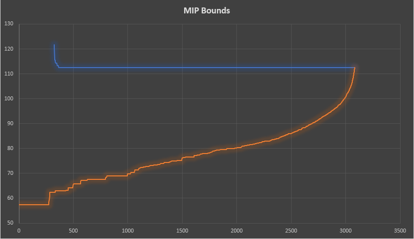
Gurobi has some real troubles with this model. After 10,000 seconds I stopped it:

    Nodes    |    Current Node    |     Objective Bounds      |     Work
 Expl Unexpl |  Obj  Depth IntInf | Incumbent    BestBd   Gap | It/Node Time

     0     0 1028.82147    0   88   -0.00000 1028.82147      -     -    0s
H    0     0                      94.1937601 1028.82147   992%     -    0s
H    0     0                     874.9562964 1028.82147  17.6%     -    0s
     0     2 1028.82147    0   88  874.95630 1028.82147  17.6%     -    0s
  5024  3355  981.36042   24   77  874.95630  989.02791  13.0%   2.4    5s
H13738 10488                     874.9564248  978.66510  11.9%   2.4    8s
 20782 16103  909.88622   55   44  874.95642  975.04173  11.4%   2.4   10s
 43494 34084  943.11968   43   57  874.95642  968.63227  10.7%   2.4   15s
 65078 50966  916.66669   49   50  874.95642  964.88315  10.3%   2.4   20s
 89405 69894  904.98150   56   44  874.95642  962.21433  10.0%   2.4   25s
 114800 89612  898.26415   51   50  874.95642  959.84933  9.70%   2.4   30s
 136964 106525  911.88894   51   49  874.95642  958.31653  9.53%   2.4   35s
 162025 125584  892.69915   52   48  874.95642  956.85312  9.36%   2.4   40s
 184525 142823  922.61714   44   57  874.95642  955.79186  9.24%   2.4   45s
 208972 161530  880.72495   54   46  874.95642  954.67328  9.11%   2.4   50s
 231067 178124  885.81556   57   44  874.95642  953.79519  9.01%   2.4   55s
 255408 196541  935.18869   46   54  874.95642  952.89911  8.91%   2.4   60s
 278680 214033  899.07410   51   47  874.95642  952.12450  8.82%   2.4   65s
 302859 232220  936.52130   37   64  874.95642  951.40827  8.74%   2.4   70s
 328028 251086  910.60834   50   50  874.95642  950.70076  8.66%   2.4   75s
 352051 268955  905.74964   54   45  874.95642  950.10317  8.59%   2.4   80s
 376120 286723  902.67637   57   43  874.95642  949.57421  8.53%   2.4   85s
 400406 304716  949.03348   26   77  874.95642  949.03348  8.47%   2.4   90s
 422676 321239  882.35938   52   47  874.95642  948.53308  8.41%   2.4   95s

. . .

 13091984 8119359  883.24548   54   44  874.95642  919.65956  5.11%   2.4 9990s
 13094401 8120718     cutoff   55       874.95642  919.65790  5.11%   2.4 9995s
 13095972 8121550  897.09522   56   41  874.95642  919.65687  5.11%   2.4 10000s
 13098502 8122984  908.84424   50   50  874.95642  919.65560  5.11%   2.4 10005s
 13100870 8124293  874.95653   56   44  874.95642  919.65388  5.11%   2.4 10010s
 13103160 8125658  883.98954   56   46  874.95642  919.65273  5.11%   2.4 10015s
 13105665 8127116  889.74823   60   40  874.95642  919.65125  5.11%   2.4 10020s
 13107878 8128361     cutoff   61       874.95642  919.64989  5.11%   2.4 10025s
 13110794 8129992  880.12914   53   48  874.95642  919.64814  5.11%   2.4 10030s
 13112818 8131096  891.49116   58   43  874.95642  919.64674  5.11%   2.4 10035s
Sending CtrlC signal

Explored 13114854 nodes (31784166 simplex iterations) in 10037.84 seconds
Thread count was 4 (of 8 available processors)

Solution count 4: 874.956 874.956 94.1938 -0

Solve interrupted
Best objective 8.749562757165e+02, best bound 9.196456216128e+02, gap 5.1076%
MIQP status(11): Optimization was terminated by the user.


Gurobi finds the optimal solution quickly but it is not able to prove optimality.

Interestingly, the global solver Baron does a very good jobs on this:

Preprocessing found feasible solution with value  0.00000000000    
 Doing local search
 Preprocessing found feasible solution with value  874.943601492    
 Solving bounding LP
 Starting multi-start local search
 Preprocessing found feasible solution with value  874.956296356    
 Done with local search
===========================================================================
  Iteration    Open nodes         Time (s)    Lower bound      Upper bound
          1             0             1.00     874.956          874.956   

 Cleaning up

                         *** Normal completion ***           

 Wall clock time:                     1.00
 Total CPU time used:                 0.75


Linearization


Let's see if we can make Gurobi look a little bit better. We can reformulate the model as a straight mixed-integer programming model:

MIP Model
\[\begin{align} \max & \sum_{i \ne j} a_i b_j y_{i,j} \\ & y_{i,j} \le x_i && \forall i \ne j \\ & y_{i,j} \le 1-x_j && \forall i \ne j \\ & 0 \le y_{i,j} \le 1 \\ & x_i \in \{0,1\} \end{align}\]

This model introduces \(100 \times 100 - 100 = 9,900\) extra continuous variables (and 19,800 additional constraints).

Derivation


We can rewrite \[\max \left(\sum_i a_i x_i \right) \left(\sum_i  b_i (1-x_i) \right) \] as \[\max \sum_{i,j} a_i b_j x_i (1-x_j)  \] We can linearize the product \[y_{i,j} = x_i (1-x_j)\] as \[\begin{align} &  y_{i,j} \le x_i \\ & y_{i,j} \le (1-x_j) \\ & y_{i,j} \ge x_i - x_j \\ & y_{i,j}, x_i \in \{0,1\}\end{align}\] You can verify the correctness of this by plugging in the possible values for \((x_i,x_j) = \{(0,0),(0,1),(1,0),(1,1)\}\). Finally we observe: 
  • \(y_{i,j}\) can be relaxed to be continuous between 0 and 1. It will be integer automatically.
  • We are really maximizing \(y_{i,j}\) so we can drop the last \(\ge\) constraints.
  • We can skip the case where \(i=j\): the product \(x_i (1-x_i)\) is always zero.

This formulation proves to be quite beneficial for Gurobi: 

    Nodes    |    Current Node    |     Objective Bounds      |     Work
 Expl Unexpl |  Obj  Depth IntInf | Incumbent    BestBd   Gap | It/Node Time

     0     0  903.79947    0  100   -0.00000  903.79947      -     -    2s
H    0     0                       2.2104609  903.79947      -     -    3s
H    0     0                     163.3432337  903.79947   453%     -    3s
H    0     0                     177.4409096  903.79947   409%     -    3s
H    0     0                     672.0256560  903.79947  34.5%     -    3s
H    0     0                     690.8350810  903.79947  30.8%     -    3s
     0     0  903.64085    0  100  690.83508  903.64085  30.8%     -    3s
H    0     0                     787.7021585  903.64085  14.7%     -    3s
     0     0  903.47324    0  100  787.70216  903.47324  14.7%     -    4s
     0     0  903.30963    0  100  787.70216  903.30963  14.7%     -    4s
     0     2  903.30963    0  100  787.70216  903.30963  14.7%     -    7s
*    4     4               2     874.9562964  888.63188  1.56%   737    9s

Cutting planes:
  Gomory: 9

Explored 7 nodes (16549 simplex iterations) in 9.53 seconds
Thread count was 4 (of 8 available processors)

Solution count 8: 874.956 787.702 690.835 ... -0

Optimal solution found (tolerance 0.00e+00)
Best objective 8.749562963561e+02, best bound 8.749562963561e+02, gap 0.0000%
MIP status(2): Model was solved to optimality (subject to tolerances).


Instead of doing this linearization by ourselves, we can also tell Gurobi to do this by using the option preqlinearize. (The behavior is not exactly the same, it solved in 12 seconds instead of 9). The automatic behavior is apparently not to apply the linearization. Too bad Gurobi does not realize it is in so much trouble and should reformulate the problem.

Cheating: a simple heuristic


We can predict the optimal solution for our specific random data set quite easily: 
  • if \(a_i\gt b_i\), set \(x_i=1\)
  • if \(a_i\lt b_i\), set \(x_i=0\)

This correctly shows the optimal solution:


----     18 heuristic solution

----     18 VARIABLE x.L  selection (binary)

i1   1.000,    i2   1.000,    i3   1.000,    i8   1.000,    i11  1.000,    i12  1.000,    i13  1.000,    i14  1.000
i19  1.000,    i20  1.000,    i21  1.000,    i25  1.000,    i26  1.000,    i28  1.000,    i34  1.000,    i37  1.000
i38  1.000,    i39  1.000,    i40  1.000,    i47  1.000,    i48  1.000,    i49  1.000,    i52  1.000,    i53  1.000
i58  1.000,    i60  1.000,    i64  1.000,    i67  1.000,    i68  1.000,    i70  1.000,    i74  1.000,    i75  1.000
i76  1.000,    i79  1.000,    i81  1.000,    i83  1.000,    i84  1.000,    i87  1.000,    i88  1.000,    i90  1.000
i91  1.000,    i92  1.000,    i94  1.000,    i96  1.000,    i98  1.000,    i100 1.000


----     18 PARAMETER count                =       46.000  number of x(i)=1
            EQUATION obj.L                 =      874.956  


Of course, this approach will only work for certain very "balanced" data sets. We exploited here that \(a_i\) and \(b_i\) are drawn from the same distribution. In addition, we have no cases where \(a_i=b_i\). I don't know about good heuristics for the more general case.

A related problem


A related problem (or better: a special case) only looks at parameter \(a\):\[\max \left(\sum_{i \in S} a_i\right) \left(\sum_{i \notin S} a_i\right) \] This problem, as noted in the comments below, has an interesting linearization. The MIQP formulation is again straightforward: \[\begin{align}\max & \left(\sum_i a_i x_i \right) \left(\sum_i  a_i (1-x_i) \right)\\ & x_i \in \{0,1\}\end{align} \] We can find the optimal solution by solving instead  \[\min \left|\sum_i a_i x_i - \sum_i  a_i (1-x_i) \right| \] I.e. make sure we divide into \(I\) into \(S\) and \(I-S\) as evenly as possible. The absolute value is easily linearized, yielding a MIP model.

Note that when we write \(A=\sum_i a_i\), we can state this as: \[\min \left| \sum_i a_i x_i - \frac{A}{2}\right|\]

Here are some performance figures for this problem:

SolverModelTimeObjGap
CplexMIQP>3600465.93140%
GurobiMIQP>3600465.93165%
BaronMIQP2465.931Optimal
CplexMIP4465.931Optimal
GurobiMIP1465.931Optimal


So we see:
  • Cplex and Gurobi do not like the MIQP model at all. They stopped on a time limit before optimality was proven. This is worse performance than on the original problem with both \(a\) and \(b\).
  • Baron does a really good job. Baron is a global NLP/MINLP solver, so it is somewhat surprising to me that it is doing so much better than more specialized MIQP solvers.
  • The MIP formulations are easy to solve.
  • The objective reported for the MIP models is not the MIP objective but rather \(\left(\sum_i a_i x_i \right) \left(\sum_i  a_i (1-x_i) \right)\) evaluated at the solution point.

The Baron log is just very convincing:


  Iteration    Open nodes         Time (s)    Lower bound      Upper bound
*         1             1             2.00     465.931          1863.72   
          1             0             2.00     465.931          465.931   


Conclusion


MIQP models, including rather smallish ones, remain very difficult to solve, even with expensive commercial solvers. The only solver that is consistently doing a good job is Baron. For most solvers it pays off to look for linearizations.   

References


Wednesday, September 19, 2018

Scheduling: Sequence Dependent Setup Times, 1 machine

The modeling of a one machine scheduling problem with sequence dependent setup times is an interesting exercise in MIP modeling.

Problem


We have \(N\) jobs to schedule. Each job has a given processing time. In addition we have a setup time for the machine in between jobs. The twist is that the required setup time depends on how two consecutive jobs differ. If two jobs in a row are very similar, the intermediate setup time is small, while if they are very different, the setup time increases. An example of such a problem is running some kind of printing jobs. Changing from a black job to a white job requires extensive cleaning, while white followed by black does not require much cleaning at all. See e.g. [1].

Some extra things to think about:

  • The last job performed (called initial below) may be important, as we may need to do a setup from the initial state to whatever the selected first job is.
  • The setup times are organized as an \((N+1) \times N\) matrix (one extra row for the initial job).
  • We can have due dates and release dates on the jobs. We need to finish a job before the due date and cannot start a job before its release date.
  • We may have some precedence relations: some jobs must be finished before another.
  • We want to sequence the jobs such that the completion time of the last job is minimized (of course subject to due date, release date and precedence constraints).

Example data


Some random data can help to understand the problem a bit better.


----     26 PARAMETER proctime  processing time

job1  2.546,    job2  8.589,    job3  5.953,    job4  3.710,    job5  3.630,    job6  3.016,    job7  4.148
job8  8.706,    job9  1.604,    job10 5.502,    job11 9.983,    job12 6.209,    job13 9.920,    job14 7.860
job15 2.176


----     26 PARAMETER setup  setup time

               job1        job2        job3        job4        job5        job6        job7        job8        job9

initial       3.559       1.638       2.000       3.676       2.741       2.439       2.406       1.526       1.600
job1                      3.010       1.641       4.490       2.060       2.143       3.376       3.891       3.513
job2          1.728                   3.243       4.080       2.191       3.644       4.023       3.510       2.135
job3          1.291       1.703                   4.001       1.712       1.137       3.341       3.485       2.557
job4          4.134       2.200       1.502                   1.277       1.808       1.020       2.078       2.999
job5          4.974       2.480       2.492       4.088                   4.652       1.478       3.942       1.222
job6          1.903       2.584       2.104       1.609       4.745                   1.539       2.544       2.499
job7          1.407       2.536       2.296       1.769       1.449       3.386                   1.180       4.132
job8          3.026       1.637       3.628       3.096       1.498       4.947       1.912                   4.107
job9          3.940       1.342       1.601       2.737       1.748       3.771       4.052       1.619
job10         1.348       3.162       1.507       3.936       1.453       2.953       4.182       2.968       3.134
job11         1.099       1.711       1.245       1.067       4.343       3.407       1.108       1.784       4.803
job12         2.573       4.222       3.164       2.563       3.231       4.731       2.395       1.033       4.795
job13         3.321       1.666       3.573       2.377       4.649       4.600       1.065       2.475       3.658
job14         2.986       1.180       4.095       3.132       3.987       3.880       3.526       1.460       4.885
job15         4.163       3.441       1.217       2.941       1.210       3.794       1.779       1.904       4.255

      +       job10       job11       job12       job13       job14       job15

initial       3.356       4.324       1.923       3.663       4.103       2.215
job1          2.855       2.653       1.471       2.257       1.186       2.354
job2          1.346       1.410       3.565       3.181       1.126       4.169
job3          2.435       1.972       1.986       1.522       4.734       2.520
job4          1.605       1.697       2.323       2.268       2.288       4.856
job5          3.305       1.206       1.024       2.605       3.080       3.516
job6          2.074       4.793       1.756       2.190       1.298       2.605
job7          4.783       3.386       3.429       2.450       3.376       3.719
job8          4.730       1.805       2.189       1.789       1.985       3.586
job9          3.782       4.383       3.451       4.904       1.108       1.750
job10                     3.175       2.805       4.901       1.735       1.654
job11         2.342                   2.037       3.563       1.621       2.840
job12         3.288       2.335                   4.066       1.440       4.979
job13         3.374       1.138       4.367                   3.032       2.198
job14         3.827       4.945       4.419       3.486                   3.804
job15         4.967       4.003       3.873       1.002       2.055


----     26 PARAMETER due  due date

job3  28.569,    job5  98.104,    job6  27.644,    job7  55.274,    job8  57.364,    job11 60.875,    job12 96.637
job13 77.888


----     26 PARAMETER release  release time

job5  19.380,    job8  48.657,    job10 27.932,    job13 24.876


----     26 SET prec  precedence restrictions

            job3

job1         YES
job2         YES


Some jobs have release and due dates. The precedence restrictions say we need to do job 1 and 2 before job 3. The setup times are displayed as a matrix: \(\mathit{setup}_{i,j}\) is the setup time between jobs \(i\) and \(j\). Notice the extra row "initial" which is the last job from the previous planning period. The diagonal elements \(\mathit{setup}_{i,i}\) are not used.

Model


To model this, I use five sets of variables:

VariableDescription
\(\color{DarkRed}{\mathit{First}}_j \in \{0,1\}\)indicates the first job
\(\color{DarkRed}{\mathit{Last}}_j \in \{0,1\}\)the last job
\(\color{DarkRed}{X}_{i,j} \in \{0,1\}\)job \(j\) immediately follows job \(i\)
\(\color{DarkRed}{\mathit{StartTime}}_j \ge 0\)the start time (after setup) of job \(j\)
\(\color{DarkRed}{\mathit{LastTime}}\)Objective variable: completion time of last job

The idea is that a job sequence \(1-2-3\) is encoded as:

  • \(\color{DarkRed}{\mathit{First}}_1=1\)
  • \(\color{DarkRed}{X}_{1,2}=\color{DarkRed}{X}_{2,3}=1\)
  • \(\color{DarkRed}{\mathit{Last}}_3=1\)

The model itself looks like:

NoEquationDescription
1\[\min \color{DarkRed}{\mathit{LastTime}}\]objective
2\[\sum_j \color{DarkRed}{\mathit{First}}_j = 1\]exactly one first job
3\[\sum_j \color{DarkRed}{\mathit{Last}}_j = 1\]exactly one last job
4\[\color{DarkRed}{\mathit{Last}}_i+\sum_{j\ne i} \color{DarkRed}{X}_{i,j} = 1\>\>\forall i\]job \(i\) is the last job or it has a successor \(j\)
5\[\color{DarkRed}{\mathit{First}}_j+\sum_{i\ne j} \color{DarkRed}{X}_{i,j} = 1\>\>\forall j\]job \(j\) is the first job or it has a predecessor \(i\)
6\[\color{DarkRed}{\mathit{StartTime}}_j \ge \color{DarkBlue}{\mathit{setup}}_{\text{initial},j} \color{DarkRed}{\mathit{First}}_j \>\>\forall j\]calculate start time of first job
7\[\color{DarkRed}{\mathit{StartTime}}_j \ge \color{DarkRed}{\mathit{StartTime}}_i + \color{DarkBlue}{\mathit{proctime}}_i + \color{DarkBlue}{\mathit{setup}}_{i,j} - M(1-\color{DarkRed}{X}_{i,j})\>\>\forall i\ne j\]calculate start time of job \(j\) with predecessor \(i\)
8\[\color{DarkRed}{\mathit{LastTime}} \ge \color{DarkRed}{\mathit{StartTime}}_j + \color{DarkBlue}{\mathit{proctime}}_j\>\>\forall j\]calculate completion time of last job
9\[\color{DarkRed}{\mathit{StartTime}}_j \ge \color{DarkBlue}{\mathit{release}}_j \>\>\forall j \]lower bound on start time
10\[\color{DarkRed}{\mathit{StartTime}}_j \le \color{DarkBlue}{\mathit{due}}_j - \color{DarkBlue}{\mathit{proctime}}_j \>\>\forall j|\color{DarkBlue}{\mathit{due}}_j>0 \]upper bound on start time
11\[ \color{DarkRed}{\mathit{StartTime}}_j \ge \color{DarkRed}{\mathit{StartTime}}_i + \color{DarkBlue}{\mathit{proctime}}_i \>\> \forall \color{DarkBlue}{\mathit{prec}}_{i,j}\]precedence constraints


In the above model I have color coded the identifiers: the variables are in red and the parameters are blue.

The big-M constant in constraint 7 was estimated by taking all processing times and adding up the largest setup times. This gives a bound on the total time we need.

Although a bit hidden from sight, this is essentially a Traveling Salesman Problem (TSP). The main issue with TSP formulations is to prevent subtours. A well-known form of subtour-elimination constraints is the Miller, Tucker, Zemlin approach [3]:

TSP Model using MTZ formulation
\[\begin{align}\min & \sum_{i\ne j} c_{i,j} x_{i,j}\\ & \sum_{j\ne i} x_{i,j} = 1 &&\forall i\\ & \sum_{i\ne j} x_{i,j} = 1 &&\forall j\\ & u_i -u_j + n x_{i,j}\le n-1 && i\ne j, i,j>1\\& x_{i,j} \in \{0,1\}, u_i \ge 0 \end{align}\]

The subtour elimination constraints can be rearranged as \[ u_j \ge u_i + 1 - n(1-x_{i,j}) \] This is now very much like equation 7.

Having explained why our formulation works, it is also clear we should not expect stellar performance. The MTZ formulation for the TSP problem is known to be rather weak. It is not surprising that scheduling models with complicated setup times are often approached with (meta) heuristics to find good solutions instead of aiming for some form of optimality.

Solution


The example data set with just \(N=15\) jobs is difficult to solve to proven optimality (takes about 3000 seconds). As usual the MIP solver finds good solutions quickly, so we can stop early if we want.

The problem itself is very small:


MODEL STATISTICS

BLOCKS OF EQUATIONS           9     SINGLE EQUATIONS          275
BLOCKS OF VARIABLES           6     SINGLE VARIABLES          257  4 projected
NON ZERO ELEMENTS         1,176     DISCRETE VARIABLES        240


Models of this size usually solve to optimality within minutes. Clearly MIP solvers perform quite poorly here. The solution looks like:


----     79 VARIABLE first.L  first job

job6 1.000


----     79 VARIABLE last.L  last job

job14 1.000


----     79 VARIABLE x.L  sequencing

             job1        job2        job3        job4        job5        job7        job8        job9       job10

job1                                1.000
job2        1.000
job4                                                                                                        1.000
job6                    1.000
job7                                                                                1.000
job10                                                                                           1.000
job11                                                                   1.000
job12                                           1.000
job15                                                       1.000

    +       job11       job12       job13       job14       job15

job3        1.000
job5                    1.000
job8                                1.000
job9                                            1.000
job13                                                       1.000


----     79 VARIABLE starttime.L  start of job (after setup)

job1   18.430,    job2    8.112,    job3   22.616,    job4   88.083,    job5   74.658,    job6    2.511
job7   43.329,    job8   48.657,    job9  102.035,    job10  93.399,    job11  32.238,    job12  79.312
job13  59.153,    job14 104.746,    job15  71.271


----     79 VARIABLE lasttime.L            =      112.607  last completion time


We can depict the solution as:


Setup and processing for each job


Each bar has two parts: the orange part indicates setup and the grey section is processing. Note again that the processing time is constant but the setup times depend on what has happened before. We see that jobs 1 and 2 are indeed processed before job 3. Jobs 3 and 6 have early due dates and we see they are processed early.

The MIP bounds are:

Lower and upper bound. The upper bound is the best found solution.

When we look at the blue line (best solution so far) we see that the solver had to do a bit of work to find a feasible integer solution. The first feasible solution was found after about 300 seconds. After that the objective quickly improved. After about 500 seconds not much was happening anymore: the solver just worked on tightening the lower bound (the best possible integer solution).

TSP relaxation


Note that if we drop the bounds related to the due and release dates and also ignore the precedence constraints, we end up with a pure TSP model. The TSP cost matrix looks like: \(c_{i,j} = \mathit{setup}_{i,j} + \mathit{proctime}_j\). The cost from the last job back to the initial job is set to zero. As expected this leads to a shorter makespan of 102.595:

Relaxed TSP solution

The orange setup times are shorter than for the original model. Of course, as the processing times are constant, we might as well use for TSP costs: \(c_{i,j} = \mathit{setup}_{i,j}\). The optimal objective value will no longer be the total makespan but the optimal sequencing will be the same.

Solving this pure TSP model with TMZ formulation is very difficult and takes much more time than the 3000 seconds we needed for the scheduling model with the additional due date, release date and precedence constraints. These extra constraints make the problem easier (which is not that surprising). To be complete: I solved the TSP model using a very different formulation from [4] (this solved very quickly for this size).


Or-tools


A very fast way of solving this model is presented in [5]. Some notes:


  • The fractional values have been scaled to make them integers. In most cases constraint solvers do not like floating point numbers. We may need to watch out for the integer range (some solver may support bigints). 
  • Preprocessing has been done to move parts of the setup time into the processing time. I.e. \[\begin{align} &\mathit{fixed}_j := \min_i \mathit{setup}_{i,j} \\  &  \mathit{proctime}_j :=  \mathit{proctime}_j  + {fixed}_j \\ & \mathit{setup}_{i,j} := \mathit{setup}_{i,j} - {fixed}_j\end{align}\] 


References


  1. A. P. Burger, C. G. Jacobs, J. H. Vuuren, S. E. Visagie, Scheduling Multi-colour Print Jobs with Sequence-dependent Setup Times, J. of Scheduling, vol. 18, no. 2, 2015, pp. 131-14
  2. Orman, A. J. and Williams, H. Paul (2004) A survey of different integer programming formulations of the travelling salesman problem. Operational Research working papers, LSEOR 04.67
  3. Miller C.E., A.W. Tucker and R.A. Zemlin (1960) Integer programming formulation of travelling salesman problems, J. ACM, 3, 326–329.
  4. Unjust benchmark: TSP MIP/Gurobi vs GA/Octave, https://yetanothermathprogrammingconsultant.blogspot.com/2009/04/unjust-benchmark-tsp-mipgurobi-vs.html
  5. https://github.com/google/or-tools/blob/master/examples/python/single_machine_scheduling_with_setup_release_due_dates_sat.py

Wednesday, September 12, 2018

LaTeX as modeling language

In [1] LaTeX is used as a modeling tool for entering Mathematical Programming models.

LaTeX as modeling language
Options

Not sure if this works well in practice. The model in the above picture was entered as:

\text{minimize} \sum\limits_{i,j}^{}(c_{i,j}x_{i,j})\\ \text{subject to:}\\ \sum\limits_{j}^{}(x_{i,j}) \leq a_{i} \quad \forall i\\ \sum\limits_{i}^{}*x_{i,j}) \geq \b_{j} \quad \forall j\\ x \in \mathbb R_+\\

Notes:
  • One of the things I am missing is: data manipulation capabilities (most of my models do serious data manipulation before I arrive at the actual model equations).
  • Large models are not easily expressed as a single LaTeX equation 
  • Reporting is missing
  • I often emphasize "readability" should be an important feature of a modeling language. Here this is taken somewhat to an extreme: the LaTeX input is fairly unreadable, while the rendered version is of course rather nice. Adding quickly a few other constraints is not so easy: it requires reading and understanding the LaTeX input.
  • Pure mathematical notation is not always unambiguous. 
  • Complex indexing structures become difficult to write in math.

References

  1. Charalampos P. Triantafyllidis, Lazaros G. Papageorgiou, An integrated platform for intuitive mathematical programming modeling using LaTeX, 2018, https://peerj.com/articles/cs-161/

Saturday, September 8, 2018

Minizinc CP/SAT vs MIP

In a previous post I discussed a simple scheduling model [1]: assign tasks to time slots subject to capacity constraints, such that we minimize the number of time slots with activity. A simple MIP model was developed for this along the lines of: \[\bbox[lightcyan,10px,border:3px solid darkblue]{\begin{align}\min& \sum_t y_t\\ & \sum_{t| \mathit{ok}_{i,t}}  x_{i,t} = 1 && \forall i \\ & \sum_{i| \mathit{ok}_{i,t}} x_{i,t} \le N && \forall t \\ & y_t \ge x_{i,t} &&\forall i,t|\mathit{ok}_{i,t}\\ & x_{i,t}, y_t \in \{0,1\}\end{align}}\] As we can see, not all task-slot combinations \((i,t)\) are allowed. The sample data set to allowed assignments is:


task_availability_map = {
    "T1" : [0, 0, 0, 1, 1, 1, 1, 1, 0, 0, 0, 0, 0, 0, 0, 0, 0],
    "T2" : [0, 0, 0, 0, 0, 1, 1, 0, 0, 0, 0, 0, 0, 0, 0, 0, 0],
    "T3" : [0, 0, 0, 1, 1, 1, 1, 1, 0, 0, 0, 0, 0, 0, 0, 0, 0],
    "T4" : [0, 0, 0, 0, 0, 1, 1, 1, 0, 0, 0, 0, 0, 0, 0, 0, 0],
    "T5" : [0, 0, 0, 0, 1, 1, 1, 1, 0, 0, 0, 0, 0, 0, 0, 0, 0],
    "T6" : [1, 1, 1, 1, 1, 1, 1, 1, 1, 1, 1, 1, 1, 1, 0, 0, 0],
    "T7" : [0, 0, 0, 0, 0, 0, 0, 0, 0, 0, 1, 1, 1, 1, 1, 0, 0],
    "T8" : [0, 0, 0, 0, 0, 0, 0, 0, 0, 0, 1, 1, 1, 1, 0, 0, 0],
    "T9" : [0, 0, 0, 0, 0, 0, 1, 1, 1, 1, 0, 0, 0, 0, 0, 0, 0],
    "T10": [0, 0, 0, 0, 0, 0, 1, 1, 1, 1, 0, 0, 0, 0, 0, 0, 0]
}

In this case we see the allowed assignments could be encoded as min, max tuples, as we have contiguous ranges. I will assume the more general case, where we only have unstructured, sparse data \(ok_{i,t}\) indicating if an assignment is allowed.


The question came up if it would be easier to formulate this as a Constraint Programming problem. There are two basic approaches we can use:


  1. Use binary variables \(x_{i,t}\). When we use a max function, we can write:\[\begin{align} \min & \sum_t \max_i \left\{ a_{i,t} x_{i,t}\right\}  \\ & \sum_t a_{i,t}  x_{i,t} = 1 && \forall i \\ & \sum_i a_{i,t} x_{i,t} \le N && \forall t \\ & a_{i,t}=0 \Rightarrow x_{i,t}=0 \\ & x_{i,t} \in \{0,1\}\end{align}\] Here \(a_{i,t}\) is our availability parameter. This generates more variables than needed. 
  2. Use binary variables but squeeze out the decision variables that we know ahead of time to be zero. This leads to \[\begin{align} \min & \sum_t \max_{i| \mathit{ok}_{i,t}} \left\{ x_{i,t} \right\} \\ & \sum_{t| \mathit{ok}_{i,t}}  x_{i,t} = 1 && \forall i \\ & \sum_{i| \mathit{ok}_{i,t}} x_{i,t} \le N && \forall t \\ & x_{i,t} \in \{0,1\}\end{align}\] This is close to the MIP model, but we do without the \(y\) variables.
  3. Use integer variables \(x_i\) to denote when task \(i\) is scheduled. \[\begin{align} \min & \sum_t \max_i \left\{ I(x_i=t) \right\} \\ & \sum_i I(x_i=t) \le N && \forall t \\&x_i \in \{t | ok_{i,t}\} \end{align}\] where \(I(.)\) is the indicator function. I.e. \[I(\delta) = \begin{cases} 1 & \text{if $\delta$ is true} \\ 0 & \text{otherwise}\end{cases}\]

First let's review the reference implementation in GAMS:

sets
  i
'task' /task1*task10/
  t
'time slot' /t1*t17/
;


*
* data
*

table allowed(i,t)
           
t1  t2  t3  t4  t5  t6  t7  t8  t9 t10 t11 t12 t13 t14 t15 t16 t17
   
task1    0   0   0   1   1   1   1   1   0   0   0   0   0   0   0   0   0
   
task2    0   0   0   0   0   1   1   0   0   0   0   0   0   0   0   0   0
   
task3    0   0   0   1   1   1   1   1   0   0   0   0   0   0   0   0   0
   
task4    0   0   0   0   0   1   1   1   0   0   0   0   0   0   0   0   0
   
task5    0   0   0   0   1   1   1   1   0   0   0   0   0   0   0   0   0
   
task6    1   1   1   1   1   1   1   1   1   1   1   1   1   1   0   0   0
   
task7    0   0   0   0   0   0   0   0   0   0   1   1   1   1   1   0   0
   
task8    0   0   0   0   0   0   0   0   0   0   1   1   1   1   0   0   0
   
task9    0   0   0   0   0   0   1   1   1   1   0   0   0   0   0   0   0
   
task10   0   0   0   0   0   0   1   1   1   1   0   0   0   0   0   0   0
;

scalar N 'capacity of a slot' /3/;

*
* derived data
*
set ok(i,t) 'set version of allowed parameter';
ok(i,t) = allowed(i,t);

scalar nok 'number of allowed assignments';
nok =
card(ok);
display nok;


*
* model
*
binary variables
  x(i,t)
'assignment'
  y(t)
'slot is used'
;
variable z 'objective variable';

equations
   assign1(i) 
'assignment constraint'
   assign2(t) 
'assignment constraint'
   ybound(i,t)
'x(i,t)=1 => y(t)=1'
   obj        
'objective'
;

assign1(i)..
sum(ok(i,t), x(i,t)) =e= 1;
assign2(t)$
sum(ok(i,t),1).. sum(ok(i,t), x(i,t)) =l= N;
ybound(ok(i,t))..  y(t) =g= x(i,t);
obj.. z =e=
sum(t,y(t));

model m /all/;

*
* solve model to optimality
*
option optcr=0;
solve m minimizing z using mip;

*
* display solution
*
option x:0,y:0,z:0;
display x.l, y.l, z.l;


Notes:

  • The parameter allowed and the set ok are stored sparsely: only the nonzero elements are stored. Each has 50 nonzero elements. For a small data set like this, this is not an issue. For larger data sets this can become very important. Note that the parameter allowed or set ok will typically come from a database or other data source. A database table will often be organized in sparse "long" format: e.g.for this case a table with columns task and slot with just 50 records. 
  • In GAMS the model size is determined by the variables that occur in the model, so the number of variables is \(n=68\) (\(x\): 50, \(y\): 17, and \(z\):1). The declaration x(i,t) does not allocate any variables.
  • The number of equations is \(m=76\)  (assign1: 10, assign2: 15, ybound: 50, obj: 1). Note that assign2 automatically skips the equations related to the "empty" columns 16 and 17 in the data table. Those columns lead to constraints of the form \(0 \le 3\). 

We have a number of issues in the model to take care of:

  • sparse data 
  • sparse \(x_{i,t}\) variables
  • empty constraints due to empty columns in the data

The GAMS model takes care of these issues automatically.

Sparsity in Minizinc


It is interesting to see what Minizinc does with a sparse model. Here is a small example:


int: N = 100;
set of int: I = 1..N;
set of int: J = 1..N;
array[I,J] of var int: x;

constraint x[1,1] = 1;
solve satisfy;

*---------------------------

Compiling sparse.mzn
Generated FlatZinc statistics:
Variables: 9999 int
Constraints: none

I somewhat expected to see a model with 1 variable and 1 constraint. We get 9999 variables: the one variable that is fixed is removed.

Other modeling tools, especially based on a programming language like Python, can create variables using loops (or list comprehensions). This allows us to skip certain variables.

Binary variable model


The easiest is just to forget about sparsity and just generate and solve fully allocated \(x_{i,t}\) model in Minizinc. This is model 1 mentioned above.


include "globals.mzn";

% number of tasks, time slots
int: ntasks = 10;
int: nslots = 17;

% sets
set of int: I = 1..ntasks;
set of int: T = 1..nslots;

array[I,T] of int: available =
   [| 0, 0, 0, 1, 1, 1, 1, 1, 0, 0, 0, 0, 0, 0, 0, 0, 0,
    | 0, 0, 0, 0, 0, 1, 1, 0, 0, 0, 0, 0, 0, 0, 0, 0, 0,
    | 0, 0, 0, 1, 1, 1, 1, 1, 0, 0, 0, 0, 0, 0, 0, 0, 0,
    | 0, 0, 0, 0, 0, 1, 1, 1, 0, 0, 0, 0, 0, 0, 0, 0, 0,
    | 0, 0, 0, 0, 1, 1, 1, 1, 0, 0, 0, 0, 0, 0, 0, 0, 0,
    | 1, 1, 1, 1, 1, 1, 1, 1, 1, 1, 1, 1, 1, 1, 0, 0, 0,
    | 0, 0, 0, 0, 0, 0, 0, 0, 0, 0, 1, 1, 1, 1, 1, 0, 0,
    | 0, 0, 0, 0, 0, 0, 0, 0, 0, 0, 1, 1, 1, 1, 0, 0, 0,
    | 0, 0, 0, 0, 0, 0, 1, 1, 1, 1, 0, 0, 0, 0, 0, 0, 0,
    | 0, 0, 0, 0, 0, 0, 1, 1, 1, 1, 0, 0, 0, 0, 0, 0, 0 |];
    
% max tasks per time slot
int: N = 3;    

array[I,T] of var 0..1: x;
var int: count;

constraint forall (i in I) ( sum([ available[i,t]*x[i,t] | t in T ] ) = 1);

constraint forall (t in T) ( sum([ available[i,t]*x[i,t] | i in I ] ) <= N );

constraint count = sum([ max([ available[i,t]*x[i,t] | i in I ]) | t in T ]);

% in this dense model we need to add:
%    available[i,t]=0 => x[i,t] = 0
constraint forall (i in I, t in T where available[i,t]=0) (x[i,t] = 0);  

solve minimize count;

Of course this is a small data set, and the standard Minizinc solvers have no problem in solving this.

It becomes a little bit more interesting with somewhat larger data set. Here is a random problem with 50 time slots and 50 tasks. The results look like:

Problem with 50 tasks and 50 time slots

Minizinc's CP solvers seem to have a big problem with this. They can not confirm the optimal solution of 17 time slots in a reasonable amount of time.

When we look at the solution in the above picture we see that the used capacity in each column is:


----     70 PARAMETER use  used capacity

t6  3,    t7  3,    t11 3,    t13 3,    t14 3,    t17 3,    t18 3,    t21 3,    t25 3,    t26 3,    t32 3,    t33 3
t34 3,    t39 3,    t44 2,    t49 3,    t50 3

All but one selected column have a used capacity of 3 (slot t44 has a count of 2). This means we will never be able to get to 16 time slots. In other words the minimum number of time slots is\[\left\lceil \frac{\mathit{ntasks}}{N}\right\rceil\] (the brackets indicate the ceiling function, i.e. rounding upwards). We can add this lower bound as an explicit constraint to the problem to help the solver. [2]

Minizinc also supports MIP solvers. The CBC MIP solver takes about 5 seconds to solve this model to optimality. Minizinc will automatically translate the max function into something the MIP solver can handle.

I have tried to implement the original squeezed binary variable model (i.e. model 2) in Minizinc. Here we try to skip all variables \(x_{i,t}\) where we know it is zero.  My version (with the small data set) looks like:


include "globals.mzn";

% number of tasks, time slots
int: ntasks = 10;
int: nslots = 17;

% sets
set of int: I = 1..ntasks;
set of int: T = 1..nslots;

% this is stored as a dense matrix
array[I,T] of int: available =
   [| 0, 0, 0, 1, 1, 1, 1, 1, 0, 0, 0, 0, 0, 0, 0, 0, 0,
    | 0, 0, 0, 0, 0, 1, 1, 0, 0, 0, 0, 0, 0, 0, 0, 0, 0,
    | 0, 0, 0, 1, 1, 1, 1, 1, 0, 0, 0, 0, 0, 0, 0, 0, 0,
    | 0, 0, 0, 0, 0, 1, 1, 1, 0, 0, 0, 0, 0, 0, 0, 0, 0,
    | 0, 0, 0, 0, 1, 1, 1, 1, 0, 0, 0, 0, 0, 0, 0, 0, 0,
    | 1, 1, 1, 1, 1, 1, 1, 1, 1, 1, 1, 1, 1, 1, 0, 0, 0,
    | 0, 0, 0, 0, 0, 0, 0, 0, 0, 0, 1, 1, 1, 1, 1, 0, 0,
    | 0, 0, 0, 0, 0, 0, 0, 0, 0, 0, 1, 1, 1, 1, 0, 0, 0,
    | 0, 0, 0, 0, 0, 0, 1, 1, 1, 1, 0, 0, 0, 0, 0, 0, 0,
    | 0, 0, 0, 0, 0, 0, 1, 1, 1, 1, 0, 0, 0, 0, 0, 0, 0 |];
    
% max tasks per time slot
int: N = 3;    

% derived data: column sums of available[i,t].
array[T] of int: sumavail = [sum([available[i,t] | i in I]) | t in T]; 
    
            
% I really want variables x[i,t] only when available[i,t]=1. 
% I don't think we can have sparse arrays. So here we
% just declare the whole thing.
array[I,T] of var 0..1: x;
var int: count;

constraint forall (i in I) ( sum([ x[i,t] | t in T where available[i,t]=1 ] ) = 1);

constraint forall (t in T) ( sum([ x[i,t] | i in I where available[i,t]=1 ] ) <= N );

constraint count = sum([ max([ x[i,t] | i in I where available[i,t]=1 ]) | t in T where sumavail[t]>=1]);

solve minimize count;

Note that the count constraints suddenly needs extra attention. The reason is that we cannot take the max of an empty list. We protected against that. A different way to do this is to add a zero to the list:

constraint count = sum([ max([0] ++ [ x[i,t] | i in I where available[i,t]=1 ]) | t in T ]);

The results for the 50 task, 50 time slot data set are:

ToolModelSizeTimeObjNodes
Minizinc/GecodeModel 1Variables: 330 int
Constraints: 144 int
> 3 hours
Minizinc/CBCModel 1Variables: 886 int, 607 float
Constraints: 420 int, 1165 float
4.5 s1710
Minizinc/CBCModel 2Variables: 885 int, 606 float
Constraints: 420 int, 1163 float
3.2 s170
GAMS/CBCMIP Modelsingle equations: 382
single variables: 334
1.2 s170

I am not sure about the Minizinc size statistics. They depend on the solver type being used: the MIP solvers need more variables. We could look at the generated "flatzinc" file which is passed on to the solver to study what is going on. (I looked at it: well, there is much going on, more than meets the eye).  I expected the size differences between model 1 and 2 using CBC to be very different, but they are very close. The solution path is also somewhat different. Not sure if I understand this.

It is interesting to see the differences in approaches between GAMS and Minizinc.

  • GAMS handles large, sparse models easily,
  • Minizinc allows some higher level modeling abstractions, such as max() and count()

Sparse data and sparse variables and constraints arise often in practical models. The fact that Minizinc does not handle sparse data and variables directly, does not mean we have to give up. E.g. the data available can  be organized in a different way:


include "globals.mzn";

% number of tasks, time slots
int: ntasks = 10;
int: nslots = 17;

% sets
set of int: I = 1..ntasks;
set of int: T = 1..nslots;
   
int: nitems = 50; 
set of int: ITEMS = 1..nitems;
array[ITEMS] of int: task = 
   [1,1,1,1,1,2,2,3,3,3,3,3,4,4,4,5,5,5,5,6,6,6,6,6,
    6,6,6,6,6,6,6,6,6,7,7,7,7,7,8,8,8,8,9,9,9,9,10,10,10,10];
array[ITEMS] of int: slot = 
  [4,5,6,7,8,6,7,4,5,6,7,8,6,7,8,5,6,7,8,1,2,3,4,5,6,7,
   8,9,10,11,12,13,14,11,12,13,14,15,11,12,13,14,7,8,9,10,7,8,9,10];
   
            
% max tasks per time slot
int: N = 3;      
            
array[ITEMS] of var 0..1: x;
var int: cnt;

constraint forall (i in I) ( sum([ x[k] | k in ITEMS where task[k]=i ] ) = 1);

constraint forall (t in T) ( sum([ x[k] | k in ITEMS where slot[k]=t ] ) <= N );

% bummer: this does not work
% constraint cnt = sum([ max([ x[k] | k in ITEMS where slot[k]=t ]) | t in T where count(slot,t)>=1]);
% work around:
array[T] of int : sumavail = [ sum([1 | k in ITEMS where slot[k]=t ]) | t in T ];
constraint cnt = sum([ max([ x[k] | k in ITEMS where slot[k]=t ]) | t in T where sumavail[t]>=1]);


solve minimize cnt;


We use here two parallel arrays task and slot to encode the sparse matrix available. Of course, we make multiple passes over the data here with these nested list comprehensions. So this becomes inefficient for very large data sets (but solvers may get into troubles then also).

Integer variable formulation


A Minizinc formulation with integer variables (model 3) can look like:

array[I] of var T: x;
var int: cnt;

constraint forall (i in I) ( x[i] in {t | t in T where available[i,t]=1 } );
constraint forall (t in T) ( count(x,t) <= N);

constraint cnt = sum( [count(x, t) >= 1 | t in T] );

solve minimize cnt;

Let's try the 50 task, 50 time slot data set. Some of the Minizinc solvers find the solution with the optimal objective cnt=17 quite quickly. But proving this is indeed the optimal solution requires to prove that a solution with cnt=16 does not exist. The CP and SAT solvers have a difficult time with this. However the built-in MIP solvers actually do a good job on this. To be able to solve this with a MIP solver Minizinc has to do some non-trivial transformations.

When we add the lower bound \[cnt \ge \left\lceil \frac{\mathit{ntasks}}{N}\right\rceil\] most solvers can prove the optimal solution in a reasonable time. The MIP solvers don't seem to need this bound: they do a good job without it.

The model above invokes the count function twice for each \(t\). We could write:


array[I] of var T: x;
array[T] of var 0..N: countx;
var int: cnt;

constraint forall (t in T) ( countx[t] = count(x,t) );

constraint forall (i in I) ( x[i] in {t | t in T where available[i,t]=1 } );

constraint cnt = sum( [ 1 | t in T where countx[t] >= 1] );

solve minimize cnt;

This does not seem to make too much different. The built-in CBC MIP solver can handle these models with ease. In [1] we see that MIP solvers can handle even sizes like 200 by 200 quite easily (that was the size suggested by the original poster).

Update


Not all solvers are created equal. Laurent Perron shows in [2] how to solve this problem very quickly using or-tools in Python (0.9 seconds). Also note the idea of adding a lower bound on the objective.

References


Appendix: 50 tasks, 50 time slots data set


% number of tasks, time slots
int: ntasks = 50;
int: nslots = 50;

% sets
set of int: I = 1..ntasks;
set of int: T = 1..nslots;

array[I,T] of int: available =
  [|0,0,0,0,0,0,0,0,1,1,1,1,1,1,1,1,0,0,0,0,0,0,0,0,0,0,0,0,0,0,0,0,0,0,0,0,0,0,0,0,0,0,0,0,0,0,0,0,0,0,
   |0,0,0,0,0,0,0,0,0,0,0,0,0,0,0,0,0,0,0,0,0,0,0,0,0,0,0,0,0,0,0,0,0,0,0,0,0,0,0,0,0,0,1,1,1,1,1,1,1,1,
   |0,0,0,0,0,0,0,0,0,0,0,0,0,0,0,0,0,0,0,0,0,0,0,0,0,0,0,1,1,1,1,1,1,1,1,0,0,0,0,0,0,0,0,0,0,0,0,0,0,0,
   |0,0,0,0,0,0,0,0,0,0,0,0,0,0,0,1,1,1,1,1,0,0,0,0,0,0,0,0,0,0,0,0,0,0,0,0,0,0,0,0,0,0,0,0,0,0,0,0,0,0,
   |0,0,0,0,0,0,0,0,0,0,0,0,0,0,1,1,1,0,0,0,0,0,0,0,0,0,0,0,0,0,0,0,0,0,0,0,0,0,0,0,0,0,0,0,0,0,0,0,0,0,
   |0,0,0,0,0,0,0,0,0,0,0,1,1,1,0,0,0,0,0,0,0,0,0,0,0,0,0,0,0,0,0,0,0,0,0,0,0,0,0,0,0,0,0,0,0,0,0,0,0,0,
   |0,0,0,0,0,0,0,0,0,0,0,0,0,0,0,0,0,1,1,1,1,1,1,1,1,0,0,0,0,0,0,0,0,0,0,0,0,0,0,0,0,0,0,0,0,0,0,0,0,0,
   |0,0,0,0,0,0,0,0,0,0,0,0,0,0,0,0,0,0,0,0,0,0,0,0,0,0,0,0,0,0,0,0,0,0,0,0,0,0,0,0,0,0,1,1,1,1,1,1,1,0,
   |0,0,0,1,1,1,0,0,0,0,0,0,0,0,0,0,0,0,0,0,0,0,0,0,0,0,0,0,0,0,0,0,0,0,0,0,0,0,0,0,0,0,0,0,0,0,0,0,0,0,
   |0,0,0,0,0,0,0,0,0,0,0,0,0,0,0,0,0,0,0,0,0,0,0,0,0,1,1,1,1,1,1,1,1,1,0,0,0,0,0,0,0,0,0,0,0,0,0,0,0,0,
   |0,0,0,0,0,0,0,0,0,0,0,0,0,0,0,0,0,0,0,0,0,0,0,0,0,0,0,0,0,0,0,0,0,0,0,0,0,0,0,0,0,0,0,0,0,0,0,0,0,1,
   |0,0,0,0,0,0,0,0,0,0,0,0,0,0,0,0,0,0,0,0,0,0,0,0,0,0,0,0,1,1,1,1,0,0,0,0,0,0,0,0,0,0,0,0,0,0,0,0,0,0,
   |0,0,0,0,0,0,0,0,0,0,0,0,0,0,0,0,0,0,0,0,0,0,0,0,0,0,0,0,0,0,0,0,0,0,0,0,0,0,0,0,0,0,0,0,0,0,0,0,0,1,
   |0,0,0,0,0,0,0,0,0,0,0,0,0,0,0,0,0,0,0,0,0,0,0,0,0,0,0,0,0,0,0,0,0,0,0,0,0,0,1,1,1,1,1,1,1,1,1,0,0,0,
   |0,0,0,0,0,0,1,1,1,1,0,0,0,0,0,0,0,0,0,0,0,0,0,0,0,0,0,0,0,0,0,0,0,0,0,0,0,0,0,0,0,0,0,0,0,0,0,0,0,0,
   |0,0,0,0,0,0,0,0,0,0,0,0,0,0,0,0,0,0,0,0,0,0,0,0,0,0,0,0,0,0,0,1,1,1,0,0,0,0,0,0,0,0,0,0,0,0,0,0,0,0,
   |0,0,0,0,0,0,0,1,1,1,1,1,1,1,0,0,0,0,0,0,0,0,0,0,0,0,0,0,0,0,0,0,0,0,0,0,0,0,0,0,0,0,0,0,0,0,0,0,0,0,
   |0,0,0,0,0,0,0,0,0,0,0,0,1,1,1,1,1,1,1,0,0,0,0,0,0,0,0,0,0,0,0,0,0,0,0,0,0,0,0,0,0,0,0,0,0,0,0,0,0,0,
   |0,0,0,0,0,0,0,0,0,0,0,0,0,0,0,0,0,0,0,0,0,0,0,0,0,0,0,0,0,0,0,0,0,1,1,1,1,1,1,0,0,0,0,0,0,0,0,0,0,0,
   |0,0,0,0,0,0,0,0,0,0,0,0,0,0,0,0,0,0,0,0,0,1,1,1,1,1,0,0,0,0,0,0,0,0,0,0,0,0,0,0,0,0,0,0,0,0,0,0,0,0,
   |0,0,0,0,0,0,0,0,0,0,0,0,0,0,0,0,0,1,1,1,1,0,0,0,0,0,0,0,0,0,0,0,0,0,0,0,0,0,0,0,0,0,0,0,0,0,0,0,0,0,
   |0,0,0,0,0,0,0,0,0,0,0,0,0,0,0,0,0,1,1,1,1,0,0,0,0,0,0,0,0,0,0,0,0,0,0,0,0,0,0,0,0,0,0,0,0,0,0,0,0,0,
   |0,0,0,0,0,0,1,1,1,1,0,0,0,0,0,0,0,0,0,0,0,0,0,0,0,0,0,0,0,0,0,0,0,0,0,0,0,0,0,0,0,0,0,0,0,0,0,0,0,0,
   |0,0,0,0,0,0,0,1,1,1,1,1,1,1,1,1,1,0,0,0,0,0,0,0,0,0,0,0,0,0,0,0,0,0,0,0,0,0,0,0,0,0,0,0,0,0,0,0,0,0,
   |0,0,0,0,0,0,0,0,0,0,0,0,0,0,0,0,0,0,0,0,0,0,0,0,0,0,0,0,0,1,1,1,1,1,1,0,0,0,0,0,0,0,0,0,0,0,0,0,0,0,
   |0,0,0,0,0,0,0,0,0,0,0,0,0,0,0,0,0,0,0,0,0,0,0,0,0,0,0,0,0,0,0,0,0,0,0,0,0,0,0,0,0,1,1,1,1,1,1,1,1,1,
   |0,0,0,0,0,0,0,0,0,0,0,1,1,1,1,1,0,0,0,0,0,0,0,0,0,0,0,0,0,0,0,0,0,0,0,0,0,0,0,0,0,0,0,0,0,0,0,0,0,0,
   |0,0,0,0,0,0,0,0,0,0,0,0,0,0,0,0,0,0,0,0,0,0,0,0,0,0,0,0,0,0,0,0,0,1,1,1,1,0,0,0,0,0,0,0,0,0,0,0,0,0,
   |0,0,0,0,0,0,0,0,0,0,0,0,0,0,0,0,0,0,0,0,0,0,0,0,0,0,0,0,0,0,0,0,0,0,0,0,0,0,1,1,1,1,1,1,1,1,0,0,0,0,
   |0,0,0,0,0,0,0,0,0,0,0,0,0,0,0,1,1,1,0,0,0,0,0,0,0,0,0,0,0,0,0,0,0,0,0,0,0,0,0,0,0,0,0,0,0,0,0,0,0,0,
   |0,0,0,0,0,1,1,1,1,0,0,0,0,0,0,0,0,0,0,0,0,0,0,0,0,0,0,0,0,0,0,0,0,0,0,0,0,0,0,0,0,0,0,0,0,0,0,0,0,0,
   |0,0,0,0,0,0,0,0,0,0,0,0,0,0,0,0,0,0,0,0,0,0,0,0,0,1,1,1,0,0,0,0,0,0,0,0,0,0,0,0,0,0,0,0,0,0,0,0,0,0,
   |0,0,0,0,0,0,0,0,1,1,1,1,1,0,0,0,0,0,0,0,0,0,0,0,0,0,0,0,0,0,0,0,0,0,0,0,0,0,0,0,0,0,0,0,0,0,0,0,0,0,
   |0,0,0,0,0,0,0,0,0,0,0,0,0,0,0,0,0,0,0,0,0,0,0,0,0,0,0,0,0,0,0,0,0,0,0,0,0,0,0,0,0,0,0,1,1,1,1,1,1,0,
   |0,0,0,0,0,0,0,0,0,0,0,0,0,1,1,1,1,0,0,0,0,0,0,0,0,0,0,0,0,0,0,0,0,0,0,0,0,0,0,0,0,0,0,0,0,0,0,0,0,0,
   |0,0,0,0,0,0,0,0,0,0,0,0,0,0,1,1,1,1,0,0,0,0,0,0,0,0,0,0,0,0,0,0,0,0,0,0,0,0,0,0,0,0,0,0,0,0,0,0,0,0,
   |0,0,0,0,0,0,0,0,0,0,0,0,0,0,0,0,0,0,0,0,0,0,0,0,0,0,0,0,0,1,1,1,1,1,0,0,0,0,0,0,0,0,0,0,0,0,0,0,0,0,
   |0,0,0,0,0,0,0,0,0,0,0,0,0,0,0,0,0,0,0,0,0,0,0,0,0,0,0,0,0,0,0,0,0,0,0,0,1,1,1,1,1,0,0,0,0,0,0,0,0,0,
   |0,0,0,0,0,0,0,0,0,0,0,0,0,0,0,0,0,0,0,0,0,0,0,0,0,0,0,0,0,0,0,1,1,1,1,1,0,0,0,0,0,0,0,0,0,0,0,0,0,0,
   |0,0,0,0,0,0,0,0,0,0,0,0,0,0,0,0,0,0,0,0,0,0,0,1,1,1,1,1,1,1,1,1,1,0,0,0,0,0,0,0,0,0,0,0,0,0,0,0,0,0,
   |0,0,0,0,0,0,0,0,0,0,0,0,0,0,0,0,0,0,0,0,1,1,1,1,1,1,1,1,1,1,0,0,0,0,0,0,0,0,0,0,0,0,0,0,0,0,0,0,0,0,
   |0,0,0,0,0,1,1,1,1,1,0,0,0,0,0,0,0,0,0,0,0,0,0,0,0,0,0,0,0,0,0,0,0,0,0,0,0,0,0,0,0,0,0,0,0,0,0,0,0,0,
   |0,0,0,0,0,0,0,0,0,0,0,0,0,0,0,1,1,1,1,1,0,0,0,0,0,0,0,0,0,0,0,0,0,0,0,0,0,0,0,0,0,0,0,0,0,0,0,0,0,0,
   |0,0,1,1,1,1,1,1,1,1,1,0,0,0,0,0,0,0,0,0,0,0,0,0,0,0,0,0,0,0,0,0,0,0,0,0,0,0,0,0,0,0,0,0,0,0,0,0,0,0,
   |0,0,0,0,0,0,0,0,0,0,0,0,0,0,0,0,1,1,1,1,1,1,0,0,0,0,0,0,0,0,0,0,0,0,0,0,0,0,0,0,0,0,0,0,0,0,0,0,0,0,
   |0,0,0,0,0,0,0,0,0,1,1,1,1,1,1,1,1,1,1,0,0,0,0,0,0,0,0,0,0,0,0,0,0,0,0,0,0,0,0,0,0,0,0,0,0,0,0,0,0,0,
   |0,0,0,0,0,0,0,0,0,0,0,0,0,0,0,0,0,0,0,0,0,0,0,0,0,0,0,0,0,0,0,0,1,1,1,0,0,0,0,0,0,0,0,0,0,0,0,0,0,0,
   |0,0,0,0,0,0,0,0,0,0,0,0,0,0,0,0,0,0,0,0,0,0,0,0,0,0,0,0,1,1,1,1,1,1,1,1,0,0,0,0,0,0,0,0,0,0,0,0,0,0,
   |0,0,0,0,0,0,0,0,0,0,0,0,0,0,0,0,0,0,0,0,0,0,0,0,0,0,0,0,0,0,0,0,0,0,0,0,0,0,1,1,1,0,0,0,0,0,0,0,0,0,
   |0,0,0,0,0,0,0,0,0,0,0,0,0,0,1,1,1,1,1,1,1,0,0,0,0,0,0,0,0,0,0,0,0,0,0,0,0,0,0,0,0,0,0,0,0,0,0,0,0,0 |];

% max tasks per time slot
int: N = 3;