Tuesday, June 28, 2016

Fantasy football

From this post:

I have been working on a hobby project for a while that involves finding all possible team rosters given the constraints of a salary cap and player positions while trying to N teams with the maximum projection. This is specifically for fantasy football, but the problem can be more generalized to a maximization problem. I can't find a more efficient solution than using nested for loops. I am using python dictionaries to track specific player data by position where qbs[playerName] = {Salary: X, Projection: Y} and rbs[playerName] = {Salary: X, Projection: Y}, etc.

The constraints are as follows:

  • 1 quarterback (qb)
  • 2 running backs (rb1, rb2)
  • 3 wide receivers (wr1, wr2, wr3)
  • 1 tight end (te)
  • 1 defense (dst)
  • 1 flex player (can be a running back, a tight end, or a wide receiver)
  • total salary has to be <= N

I assume the two N’s in this description are different: one is the salary cap, the other is the number of solutions to be found. Let’s try to generate some random data:

image

I just generate 25 candidate players: 5 candidate players for each 5 positions. This is stored in the set \(plpos_{pl,pos}\).

The basic model for one best solution is as follows:

image

Note that we don’t strictly need the \(y\) variables. We can substitute them out (or relax them to continuous variables).

I assume we want to generate 10 solutions (see set \(sols\) below). The idea to find the 10 best solutions is to implement the following algorithm:

1. Solve MIP
2. If enough solutions: STOP
3. Add a constraint (cut) to the model that forbids the current solution
4. Go to step 1.

In the code below the cuts are expressed in equation \(cut_{sol}\), where \(sol\) is a dynamic set that grows each iteration. We start with the empty set: \(sol:=\emptyset\).

image

Usually the cut to prevent an earlier found binary solution vector \(x^*_i\) is as follows:

\[ \sum_{i|x^*_i=1} x_i -\sum_{i|x^*_i=0} x_i \le n-1 \]

where \(n\) is the number of \(x^*_i=1\). For a derivation see here. In our case we know \(\sum x_i=n\) so we can use a simpler cut:

\[ \sum_{i|x^*_i=1} x_i  \le n-1 \]

The algorithm looks like:

image

Because in integer programming we can see solution values like 0.99999, we just consider all values \(>0.5\) as one. When we run this code we see:

image 
All 10 solutions obey the salary cap. The total projection (the objective) is slowly getting worse when we search for new solutions.

It is noted that some solvers provide tools to generate “next best” solutions more efficiently (e.g. Cplex’s solution pool).

I was pointed towards a related approach documented in this paper (1). I did not read it: the publisher charges $50 to download the pdf file (for 13 pages that is $3.85 per page, beating this paper).

References

(1) Andrew C. Trapp and Renata A. Konrad, Finding diverse optima and near-optima to binary integer programs, IIE Transactions, 47 (11), 2015, pp.1300-1312.

Monday, June 20, 2016

More tennis scheduling

Centre Court.jpgIn this post another tennis-scheduling problem is posted. In this case we deal with 20 players doing doubles in 5 rounds. That means teams of 2 players, 4 players per game, and 5 games per round.

Restriction 1

The first restriction is that a player \(i\) and player \(j\) can be team-members only once. I.e. they can play together zero or one time. There is no restriction on how many times player \(i\) can meet player \(j\) as opponent.

Restriction 2

Each player has a rating or level between 1 and 5. The level of a team is the sum of the ratings of the two players.  We don’t want the level of two opposing teams to differ by more than 1.5.

The Model

tennis3a

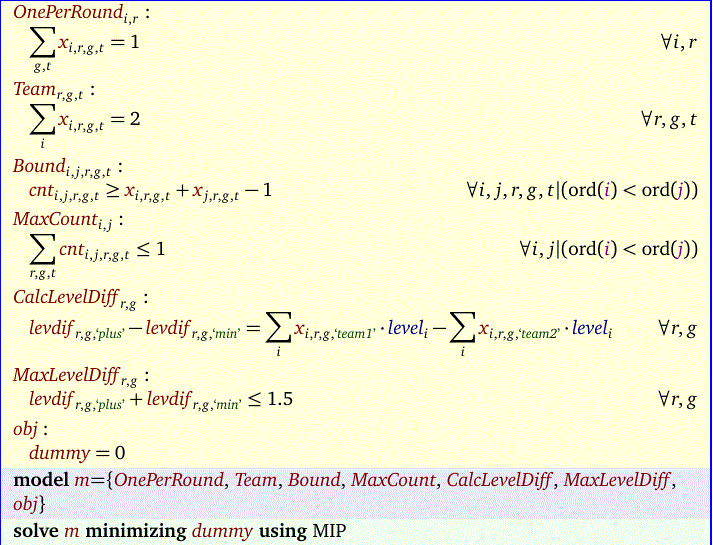
The main variable is \(x_{i,r,g,t}\) which indicates if player \(i\) is playing in round \(r\), game \(g\) in team \(t\).

The level difference restriction:\[\max_{i<j} \sum_{r,g,t} x_{i,r,g,t} x_{j,r,g,t} \le 1\] is not completely trivial to linearize. The idea is to linearize the inner product by introducing additional variables \(cnt_{i,j,r,g,t}\). Then we just sum these. Note that \(cnt_{i,j,r,g,t}\) can be considered a binary variable. I relaxed that here to a positive continuous variable (you may verify this is allowed here).

The difference in level of two opposing teams is implemented using a standard variable splitting technique. We used random player levels.

tennis3b

The final solution is:

tennis3c

It is noted that instead of a bound on the level difference, we also could minimize this quantity (allowing for even better matchups where possible).

Sunday, June 19, 2016

Filling up a container with boxes

In this post the following problem was proposed:

We have a rectangular container in which we pace some differently sized boxes (rectangles, this problem is 2D only). There is some space left, and we want to fill that with as many standard sized boxes as possible.

image

Here the yellow boxes are the original pay load and the blue boxes are the ones we were able to add. Note that we are allowed to rotate the rectangles.

This can be formulated by a Mixed Integer Programming or a Constraint Programming model. The main ingredient is a set of ‘no-overlap’ constraints. Here is some background information about these constraints. In our case things are slightly more complex as we allow 90° rotation.

Variables

The decision variables we use are as follows:

image

The variables \(q_{i,c}\) are not really needed (we can recalculate them from \(p_{i,c}\) and \(u_{i,r}\) when needed) but they help to simplify a number of constraints.

Equations

image

The model is not extremely complicated, although the rotation needs attention.

To get better performance we can add some symmetry-breaking constraints and use some branching priorities. Even then proving optimality is very difficult. However a good MIP solver will find very good solutions very quickly.

Saturday, June 18, 2016

Solving non-convex QP problems as a MIP

Non-convex Quadratic Programming problems are difficult to solve to optimality. Most QP solvers do not even accept non-convex problems, so how can we attack this?

The easy way: global solvers

The easiest is just to use a global solver. We can use global NLP solvers such as Baron, Qouenne or Antigone. In addition Cplex has a solver for non-convex QP and MIQP problems (you need to set an option for this: OptimalityTarget = 3; Cplex will not automatically use this non-convex solver). For these solvers make sure to set the gap tolerance (GAMS option OPTCR) to zero.

Theory: KKT Conditions

A QP model can look like:

\[\begin{align}\min\>\>  & c^Tx + x^TQx \\
&Ax \le b\\
& \ell \le x \le u \end{align}\]

The KKT conditions for this QP are:

\[\begin{align} & 2Qx + c - A^T\mu – \lambda - \rho = 0\\
&(Ax – b)^T\mu = 0\\
&(x-\ell)^T\lambda = 0 \\
&(x-u)^T\rho = 0\\
& \ell \le x \le u \\ & Ax \le b \\
& \lambda \ge 0,\rho \le 0, \mu \le 0 \end{align}\]

There are two complications with this LCP (Linear Complementarity Problem):

  • The complementarity conditions \((Ax – b)^T\mu\), \((x-\ell)^T\lambda=0\) and  \((x-u)^T\rho\) are not linear and can not be used directly in an LP or MIP model
  • There are likely multiple solutions, so we need a way to select the best

A MIP formulation

To make the above model amenable to a linear solver we first try to linearize the complementarity conditions. Let’s consider \((x-\ell)^T\lambda=0\). This can be attacked as follows. The condition \((x_i –\ell_i)\lambda_i = 0\) really means \(x_i=\ell_i\) or \(\lambda_j=0\). This can be linearized as:

\[\begin{align} & x_i  \le \ell_i +M \delta_i\\
& \lambda_i  \le M (1-\delta_i) \\
& \delta_i \in \{0,1\} \end{align}\]

We can do something similar for \((x-u)^T\rho\) and \((Ax – b)^T\mu \).

The big-M coefficient are a problem of course. We either need to find some good values for them or use a formulation that does not need them. Some techniques that could help here are SOS1 (Special Order Sets of Type 1) variables where each combination \(y_i, \lambda_i\) (where \(y_i=x_i-\ell_i\) forms a SOS1 set. An alternative is to use some indicator variables (these are supported by a number of solvers).

The second issue is to find the best solution. Obviously we could add an objective \(\min\> c^Tx + x^TQx\) but that makes the problem non-linear again. It turns out that \(c^Tx + x^TQx = \frac{1}{2} \left[ c^Tx +\ell^T\lambda + u^T\rho+ b^T\mu\right]\). This is now a linear objective!

Objective

The derivation of the linear objective is as follows:

\[\begin{align} & c^Tx + x^TQx\\
= \>& c^Tx + \frac{1}{2} x^T ( \lambda + \rho + A^T\mu – c)\\
= \> & c^Tx + \frac{1}{2}x^T\lambda + \frac{1}{2}x^T\rho + \frac{1}{2}(Ax)^T\mu – \frac{1}{2}x^Tc\\
=\> & \frac{1}{2} c^Tx + \frac{1}{2}\ell^T\lambda + \frac{1}{2}u^T\rho + \frac{1}{2} b^T\mu \end{align}\]

It is quite fortunate that we are able to get rid of the quadratic term and form a linear objective.

Example: Non-convex QP

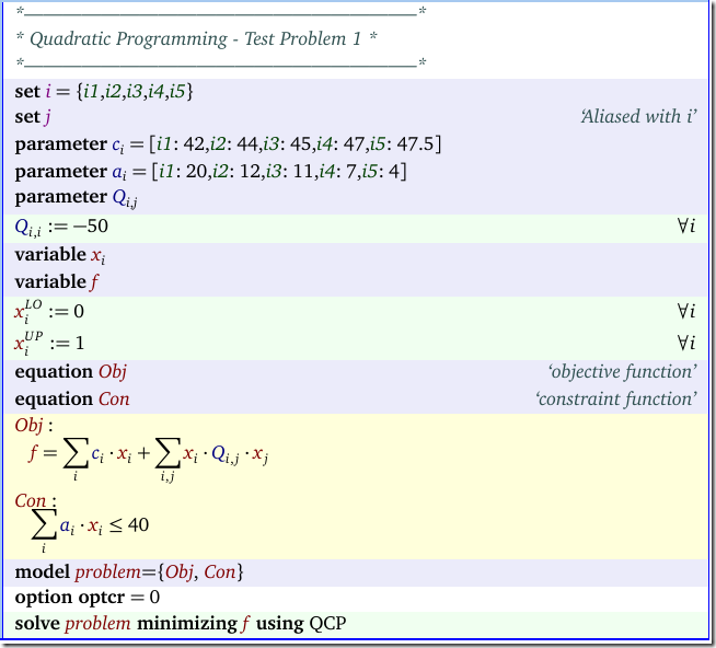
A simple example is from (1):

image

Solving this directly gives:

                           LOWER          LEVEL          UPPER         MARGINAL

---- EQU Obj                 .              .              .             1.0000     
---- EQU Con               -INF           39.0000        40.0000          .         

  Obj  objective function
  Con  constraint function

---- VAR x 

          LOWER          LEVEL          UPPER         MARGINAL

i1          .             1.0000         1.0000       -58.0000     
i2          .             1.0000         1.0000       -56.0000     
i3          .              .             1.0000        45.0000     
i4          .             1.0000         1.0000       -53.0000     
i5          .              .             1.0000        47.5000     

                           LOWER          LEVEL          UPPER         MARGINAL

---- VAR f                 -INF          -17.0000        +INF             .         


Example: MIP with big-M coefficients

We name our duals as follows:

\[\begin{align}
x_i \ge \ell_i & \perp  \lambda_i \ge 0 \\
x_i \le u_i & \perp  \rho_i \le 0 \\
\sum_i a_i x_i \le b & \perp \mu \le 0
\end{align}\]

The complete model looks like:

image

image

The results look like:

                           LOWER          LEVEL          UPPER        

---- VAR f                 -INF          -17.0000        +INF                     

---- VAR x 

          LOWER          LEVEL          UPPER        

i1          .             1.0000         1.0000            
i2          .             1.0000         1.0000            
i3          .              .             1.0000            
i4          .             1.0000         1.0000            
i5          .              .             1.0000            

---- VAR lambda  dual of x.lo

          LOWER          LEVEL          UPPER        

i1          .              .            +INF                      
i2          .              .            +INF                      
i3          .            45.0000        +INF                      
i4          .              .            +INF                      
i5          .            47.5000        +INF                      

---- VAR rho  dual of x.up

          LOWER          LEVEL          UPPER        

i1        -INF          -58.0000          .                       
i2        -INF          -56.0000          .                       
i3        -INF             .              .                       
i4        -INF          -53.0000          .                       
i5        -INF             .              .                       

                           LOWER          LEVEL          UPPER        

---- VAR mu                -INF             .              .                      

  mu  dual of a*x<=b

---- VAR delta 

             LOWER          LEVEL          UPPER        

lo.i1          .             1.0000         1.0000            
lo.i2          .             1.0000         1.0000            
lo.i3          .              .             1.0000               
lo.i4          .             1.0000         1.0000            
lo.i5          .              .             1.0000               
up.i1          .              .             1.0000               
up.i2          .              .             1.0000               
up.i3          .             1.0000         1.0000            
up.i4          .              .             1.0000               
up.i5          .             1.0000         1.0000            

                           LOWER          LEVEL          UPPER        

---- VAR gamma               .             1.0000         1.0000            


For some performance comparisons see (3).

References

(1)  Floudas e.a., Handbook of Test Problems in Local and Global Optimization, Kluwer, 1999.
(2)  Wei Xia, Juan Vera, Louis F. Zuluaga, Globally Solving Non-Convex Quadratic Programs via Linear Integer Programming Techniques, report, Nov 17, 2015.
(3)  http://yetanothermathprogrammingconsultant.blogspot.com/2016/07/non-convex-qp-as-mip-performance.html

Thursday, June 16, 2016

GAMS + R: retrieving online WB data

https://www.jgea.org/resources/jgea/ojs/index.php/jgea/article/view/22/6

image

Notes:

  • csv2gdx and gdxrrw are other possible tools to get data from R into GAMS
  • Using CSV files, one may encounter some internationalization issues (decimal point vs comma etc.)

Tuesday, June 14, 2016

Getting GAMS data into Julia

Using gdx2sqlite it is very easy to populate a SQLite database from GAMS data. This should allow us to get data into Julia somewhat painlessly. Let's try:


Formatting of Data.Tables

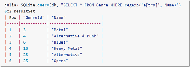
Interestingly the format of the Data.Table is not as nice as advertised in https://github.com/JuliaDB/SQLite.jl, where we see:

image

I get rather ugly output, not a nicely formatted table. The trick seems to be to convert the Data.Table into a DataFrame. Note that it is important to import the DataFrames package before SQLite.

Monday, June 13, 2016

Loops considered harmful

In many interpreted languages, the use of loops is discouraged, and “vectorized” implementations are preferred. This is the case for Matlab, R, Python and also GAMS. There are two main reasons:

  • loopless code has less clutter, and may be easier to write and read.
  • vectorized code performs often much better.

Here is an example:

Sets
    i   
/1*5/
   
alias(i,j);

Parameters

    c(i)
   
/1    42
    
2    44
    
3    45
    
4    47
    
5    47.5/
    Q(i,j);

loop(i, loop(j, Q(i,j) = 100 $ (ord(i) eq ord(j))));

Variables
    x(i)
    f;

loop
(i,
    x.lo(i) = 0;
    x.up(i) = 1);


The first construct sets the diagonal of Q to 100. This really should be written as:

Q(i,i) = 100;

One could read this as an “implicit loop”. Similarly in the second construct we can drop the explicit loop and just write:

x.lo(i) = 0;
x.up(i) = 1
;

Timings

The loop used to populate the diagonal of the matrix Q is really the worst possible way to express this. Here are some suggestions for improvement:

  • Replace loop(i, loop(j, by loop((i,j),  This does not make a difference in performance but it looks better.
  • Put the $ condition on the left side of the assignment: loop((i,j), Q(i,j)$(ord(i)=ord(j)) = 100); This will improve the performance a lot. The result of putting the $ on the left is that we assign diagonal elements only, instead of assigning all elements.  
  • Put the $ condition on the loop sets: loop((i,j)$(ord(i)=ord(j)), Q(i,j) = 100); This is even faster than the previous version.
  • Finally use an implicit loop: Q(i,i) = 100;. This is the most readable and also the fastest.

The speed difference in the assignment of Q for a set i of size 2000 is remarkable:

Formulation n=2000, time in seconds Code
1. Original formulation 30 loop((i,j), Q(i,j) = 100$(ord(i)=ord(j)));
2. Loop with dollar condition on the LHS 1.2 loop((i,j), Q(i,j)$(ord(i)=ord(j)) = 100);
3. Loop with dollar condition on the loop set 0.6 loop((i,j)$(ord(i)=ord(j)), Q(i,j) = 100);
4. Vectorized 0 Q(i,i) = 100;
Note: $ Conditions

To be complete, let’s detail how the GAMS $ condition works when placed left or right of the assignment. The construct

   a(i)$s(i) = 1

means if s(i)=true then assign a(i)=1.

Opposed to this,

    a(i) = 1$s(i)

means if s(i)=true then assign a(i)=1 else assign a(i)=0.

I seldom use the second form while I use the $ on the left all the time. This example shows this is with good reason.

New version of CMPL

From this post :

CMPL( Mathematical Programming Language) is a mathematical programming language and a system for mathematical programming and optimisation of linear optimisation problems.

The CMPL syntax is similar in formulation to the original mathematical model but also includes syntactic elements from modern programming languages. CMPL is intended to combine the clarity of mathematical models with the flexibility of programming languages.

New main features and change log :

Coliop4
Coliop4 is the new GUI for CMPL available on Window, Linux and Mac.
It is more comfortable and flexible and comes with syntax highlighting.

Installation
An installation is not longer necessary. The entire CMPL package runs now out of the box in every directory.

pyCmpl and CmplServer
A couple of bottlenecks were identified and cleaned. Therefore the performance is considerably increased.

Cmpl
Some minor bugs were found and fixed.

SolverStudio
Cmpl has been part of SolverStudio since last year. The performance of the Cmpl plug-in in SolverStudio is considerably increased.

For more information please visit www.coliop.org and projects.coin-or.org/Cmpl.

Tuesday, June 7, 2016

Optimizing some R code

I have a somewhat largish data set with \(n=5291\) rows:

> str(df)
'data.frame':	5291 obs. of  5 variables:
 $ ID         : int  1 2 3 4 5 6 7 8 9 10 ...
 $ Performance: num  0.705 0.707 0.709 0.711 0.713 ...
 $ Cost       : int  4365766 4366262 4367526 4368147 4369411 4372412 4372908 4374172 4374793 4376057 ...
 $ Weight     : int  49595 50335 51091 50242 50998 53125 53865 54621 53772 54528 ...
 $ Distance   : num  0.997 0.991 0.987 0.957 0.953 ...

Three of the columns indicate objectives of an underlying optimization problem: Cost, Weight and Performance. The rows correspond to the Pareto optimal set.

In (1) an algorithm is shown to find a subset, called k-optimal solutions. For this we need to calculate the following. First define a function \(\Gamma(v)\) which compares one objective function value \(k\) between two different points \(i\) and \(j\). Let’s assume minimization for all objectives, then we have:

\[\Gamma(v)=\begin{cases} 0 & \>\text{if $v>0$}\\ 1 & \>\text{if $v\le 0$} \end{cases} \]

Basically it says that \(v=f_i^k-f_j^k\), \(\Gamma(v)=1\) if objective \(k\) in point \(i\) is better (or the same) than the corresponding objective in point \(j\) and \(\Gamma(v)=0\) otherwise. The goal of this exercise is to calculate a matrix

\[K_{i,j} =  \sum_k \Gamma(f_i^k-f_j^k) – 1\]

Obviously this is an operation that is quadratic in \(n\).

We have another small vector objs that as the objective names and the direction (\(1\)=minimize, \(-1\)=maximize):

> objs
Performance        Cost      Weight 
         -1           1           1 

Attempt 1: use the data frame directly

The first try, just operates on the data frame df directly.

# allow to be called with smaller n
calcK1 <- function(n=nrow(df)) {
 
  gamma <- function(i,j,k) {
    v <- objs[k]*(df[i,k] - df[j,k])
    if (v>0)
      0L
    else
      1L
  }
 
  K<-matrix(0L,n,n)
  for (i in 1:n) {
    for (j in 1:n)
      if (i!=j) K[i,j] <- sum(sapply(names(objs),function(k) gamma(i,j,k))) – 1L
  }
  K
}

We try for different subsets of \(n\):

size \(n\) time (sec)
50 0.9
100 3.7
150 8.3
200 14.9
5291 2.9 hours (estimated)

That is really terrible.

Attempt 2: use a matrix

One bottleneck could be the use of a data frame. The most inner loop jumps from one column to the next, and that is a relatively expensive operation. Let’s try to convert the data first to a matrix and then operate on the matrix:

calcK2 <- function(n=nrow(df)) {
 
  # calculate matrix A
  m <- length(objs)
  A <- matrix(0,n,m)
  k <- 0L
  for (c in names(objs)) {
    k <- k + 1L
    A[,k] <- df[1:n,c]*objs[c]
  }

  gamma <- function(i,j,k) {
    if ((A[i,k] - A[j,k])>0)
      0L
    else
      1L
  }
 
  sumgamma <- function(i,j) {
    s <- 0L
    for (k in 1:m) {
      s <- s + gamma(i,j,k)
    }
    s-1L
  }
 
  K<-matrix(0L,n,n)
  for (i in 1:n) {
    for (j in 1:n)
      if (i!=j) K[i,j] <- sumgamma(i,j)
  }
  K
}

This is much better:

size \(n\) time (sec)
50 0.06
100 0.25
150 0.58
200 1.03
5291 0.2 hours (estimated)

To get better performance we should get rid of these loops somehow. In R loops are very slow. In C++ loops don’t have this disadvantage, so instead of trying to vectorize this (besides I don’t see immediately how), let’s use some C++ code.

Attempt 3: use some C++ code

The Rcpp package makes it very easy to develop C++ functions for use inside R. We assume again we first make a matrix \(A\). The C++ code looks like:

#include <Rcpp.h>
using namespace Rcpp;

// [[Rcpp::export]]
IntegerVector calcKcpp(NumericVector A, int n, int nk) {

  IntegerVector K(n*n); // will be initialized to zero
  for (int i=0; i<n; ++i)
    for (int j=0; j<n; ++j)
      if (i!=j) {
        int s = 0;
        for (int k=0; k<nk; ++k)
          if (A[k*n+i]<=A[k*n+j])
            ++s;

        K[j*n+i] = s-1;
      } 
  return K;
}

Note that R matrices are stored column-wise (the old Fortran way). We use this function as follows:

Rcpp::sourceCpp('c:/tmp/kepsilon/kepsc.cpp')

calcK3 <- function(n=nrow(df)) {

  # calculate matrix A
  m <- length(objs)
  A <- matrix(0,n,m)
  k <- 0L
  for (c in names(objs)) {
    k <- k + 1L
    A[,k] <- df[1:n,c]*objs[c]
  }
 
  # call C++ code
  K <- calcKcpp(A,n,m)
  dim(K) = c(n,n)
  K
}

The timings are now:

size \(n\) time (sec)
50 0
100 0
150 0
200 0
5291 0.9 seconds

This is more than fast enough to allow for some experimentation with this data set.

Comparison: computation in GAMS

Here we do the same computation in GAMS.

sets
  i
/1*5291/
  obj
/performance,weight,cost/
;
alias (i,j);

parameter d(i,obj) 'data'
;
$gdxin testsolution.gdx
$loaddc d

parameter objmin(obj) /performance -1, weight 1, cost 1/
;

* make all objectives minimization

d(i,obj) = objmin(obj)*d(i,obj);

parameter
K(i,j);
K(i,j)$(
ord(i)<>ord(j)) = sum
(obj$(d(i,obj)<=d(j,obj)),1)-1;

The time needed for the full problem is:

size \(n\) time (sec)
5291 34 seconds

GAMS is actually doing very well on this.
References

(1) Gobbi, Massimiliano. 2013. “A K, K-\(\varepsilon\) Optimality Selection Based Multi Objective Genetic Algorithm with Applications to Vehicle Engineering.” Optimization and Engineering 14 (2). Springer: 345–60. doi:10.1007/s11081-011-9185-8.