Showing posts with label tsp. Show all posts

Friday, August 4, 2023

Some TSP MTZ experiments

In [1], a question was posed about a TSP model using the MTZ (Miller-Tucker-Zemlin) subtour elimination constraints. The results with Julia/glpk were disappointing. With \(n=58\) cities, things were taken so long that the solver seemed to hang. Here I want to see how a precise formulation with a good MIP solver can do better. As seeing is believing, let's do some experiments. 

The standard MTZ formulation[1] can be derived easily. We use the binary variables \[\color{darkred}x_{i,j}=\begin{cases}1 & \text{if city $j$ is visited directly after going to city $i$}\\ 0 & \text{otherwise}\end{cases}\]  

Friday, December 11, 2020

Electronic Amoeba for solving TSPs?


Abstract

Combinatorial optimization to search for the best solution across a vast number of legal candidates requires the development of a domain-specific computing architecture that can exploit the computational power of physical processes, as conventional general-purpose computers are not powerful enough. Recently, Ising machines that execute quantum annealing or related mechanisms for rapid search have attracted attention. These machines, however, are hard to map application problems into their architecture, and often converge even at an illegal candidate. Here, we demonstrate an analogue electronic computing system for solving the travelling salesman problem, which mimics efficient foraging behaviour of an amoeboid organism by the spontaneous dynamics of an electric current in its core and enables a high problem-mapping flexibility and resilience using a resistance crossbar circuit. The system has high application potential, as it can determine a high-quality legal solution in a time that grows proportionally to the problem size without suffering from the weaknesses of Ising machines.

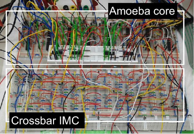
Picture of the electronic amoeba (from [2])


"Electronic amoeba" sounds awful. Furthermore, the paper talks about "legal solutions". Now the lawyers even get involved... 
 

References

  1. 'Electronic amoeba' finds approximate solution to traveling salesman problem in linear time, https://www.sciencedaily.com/releases/2020/12/201210112050.htm
  2. Kenta Saito, Masashi Aono and Seiya Kasai, Amoeba-inspired analog electronic computing system integrating resistance crossbar for solving the travelling salesman problem, https://www.nature.com/articles/s41598-020-77617-7


Monday, February 10, 2020

Longest path problem


This is a question that regularly pops up: how to solve the longest path problem? At first sight, this is easy. Just replace the "minimize" in the shortest path problem by "maximize" and we are good to go. Unfortunately, opposed to the well-known shortest path problem, the longest path problem is not that easy to state and to solve.

1. Standard Shortest Path Formulation


The standard shortest path can be formulated as a Mixed Integer Programming problem:

Shortest Path Problem
\[\begin{align} \min& \sum_{(i,j)\in\color{darkblue} A} \color{darkblue}d_{i,j} \color{darkred}x_{i,j} \\ & \sum_{j|(j,i)\in \color{darkblue}A} \color{darkred}x_{j,i} + \color{darkblue}b_i = \sum_{j|(i,j)\in \color{darkblue}A} \color{darkred}x_{i,j} && \forall i \\ &\color{darkred}x_{i,j} \in \{0,1\} \\ & \color{darkblue} b_i = \begin{cases}1 & \text{if $i$ is a source node} \\ -1 & \text{if $i$ is a sink node} \\ 0 & \text{otherwise} \end{cases} \end{align} \]

where \(A\) is our network and \(b\) is a sparse data vector indicating the exogenous inflow or outflow at the source or sink node.

Network with the shortest path

There are some implicit assumptions in this model: there are no negative cycles. In the above example, \(d_{i,j}\) represents distance, so we have \(d_{i,j}\ge 0\) and there is no problem of negative cycles.

Shortest path problems are very easy MIPs to solve. The solution is automatically integer, so it can be solved as an LP and these LPs are very sparse (only two non-zero elements per column) and very easy to solve. In addition, specialized network solvers are widely available.

The problem in the picture has 20 nodes and 37 × 2 arcs. In this example, the arcs are duplicated to make sure we can go in two directions. This leads to an LP of 74 variables and 20 constraints. The solution looks like:


----     75 VARIABLE z.L                   =      128.538  objective

----     75 VARIABLE x.L  flow

            point6(B)     point15     point16     point18     point20

point5(A)                               1.000
point15         1.000
point16                                             1.000
point18                                                         1.000
point20                     1.000


2. Just use max


When we just turn the above problem in a maximization problem, we get results that are difficult to interpret. But they certainly don't form what we would call a path:


----     78 VARIABLE z.L                   =     1638.406  objective

----     78 VARIABLE x.L  flow

               point1      point2      point3      point4   point5(A)   point6(B)      point7      point8      point9

point1                                              1.000
point3                                                                                                          1.000
point4          1.000
point5(A)                                                                                           1.000
point6(B)                                                                               1.000
point7                                                                      1.000
point8                                                          1.000
point9                                  1.000
point10                     1.000
point12                                                                                                         1.000
point13                                                                                 1.000
point14                                             1.000                                           1.000
point15                                                                     1.000
point16                                                                                             1.000
point17         1.000                               1.000
point18                                 1.000                                                                   1.000
point19                                                                                 1.000
point20                     1.000

        +     point10     point11     point12     point13     point14     point15     point16     point17     point18

point1                                                                                              1.000
point2          1.000
point3                                                                                                          1.000
point4                                                          1.000                               1.000
point5(A)                                                                               1.000
point7                                              1.000
point8                                                          1.000                   1.000
point9                                  1.000                                                                   1.000
point10                                                                     1.000
point11                                                                                                         1.000
point12                                                                                 1.000                   1.000
point14                                                                                 1.000       1.000
point15         1.000
point16                                 1.000                   1.000                               1.000       1.000
point17                                                         1.000                   1.000                   1.000
point18                     1.000       1.000                                                       1.000
point19                                             1.000                   1.000                   1.000       1.000
point20         1.000       1.000                   1.000                   1.000

        +     point19     point20

point2                      1.000
point7          1.000
point10                     1.000
point11                     1.000
point13         1.000       1.000
point15         1.000
point17         1.000
point18         1.000       1.000
point19                     1.000
point20         1.000

Maximization results

Basically, all but a few lines in the plot are traveled in both directions. Conclusion: this is not what we are looking for.

3. TSP-like solution


To form a proper path (called an elementary path), we need to add two sets of constraints [1]:
  1. The outflow of each node goes to just one arc: \[\sum_{j|(i,j)\in A} x_{i,j} \le 1\>\forall i\]
  2. Forbid any sub-tours to be formed. Sub-tour elimination constraints are well-known from the Traveling Salesman Problem. 
Using the simple MTZ (Miller, Tucker, and Zemlin) approach, we can formulate:


Longest Path Problem
\[\begin{align} \max& \sum_{(i,j)\in\color{darkblue} A} \color{darkblue}d_{i,j} \color{darkred}x_{i,j} \\ & \sum_{j|(j,i)\in \color{darkblue}A} \color{darkred}x_{j,i} + \color{darkblue}b_i = \sum_{j|(i,j)\in \color{darkblue}A} \color{darkred}x_{i,j} && \forall i \\ & \sum_{j|(i,j)\in \color{darkblue}A} \color{darkred}x_{i,j} \le 1 && \forall i\\ & \color{darkred}t_j \ge \color{darkred}t_i + 1 + (\color{darkblue}n-1)(\color{darkred}x_{i,j}-1) && \forall i,j|i\ne\text{source},j\ne\text{sink} \\&\color{darkred}x_{i,j} \in \{0,1\} \\ & \color{darkred}t_i \ge 0  \end{align} \]

Here \(n\) is the number of nodes.

The results look like:


----    126 VARIABLE z.L                   =      432.987  objective

----    126 VARIABLE x.L  flow

               point1      point2      point3      point4   point6(B)      point7      point8      point9     point10     point12

point2                                                                                                          1.000
point4          1.000
point5(A)                                                                               1.000
point9                                  1.000
point12                                                                                             1.000
point14                                             1.000
point15                                                         1.000
point16                                                                                                                     1.000
point19                                                                     1.000
point20                     1.000

        +     point13     point14     point15     point16     point17     point18     point19     point20

point1                                                          1.000
point3                                                                      1.000
point7          1.000
point8                      1.000
point10                                 1.000
point13                                                                                             1.000
point17                                             1.000
point18                                                                                 1.000

Solution of Longest Elementary Path Model


This looks much better.

More formulations can be found in [1].

4. Ad-hoc approach


Let's drop the sub-tour elimination constraints, and have a look at the solution of the remaining model:


Problem A: drop sub-tour elimination constraints
\[\begin{align} \max& \sum_{(i,j)\in\color{darkblue} A} \color{darkblue}d_{i,j} \color{darkred}x_{i,j} \\ & \sum_{j|(j,i)\in \color{darkblue}A} \color{darkred}x_{j,i} + \color{darkblue}b_i = \sum_{j|(i,j)\in \color{darkblue}A} \color{darkred}x_{i,j} && \forall i \\ & \sum_{j|(i,j)\in \color{darkblue}A} \color{darkred}x_{i,j} \le 1 && \forall i\\ &\color{darkred}x_{i,j} \in \{0,1\}  \end{align} \]

When we look at the solution we see a number of sub-tours of just two points. This means: travel from \(C\rightarrow D\) and back.

Sub-tours with 2 points


These special sub-tours are easily prevented: add a cut of the form \[x_{i,j}+x_{j,i} \le 1\] We can add them only for the \(i \rightarrow j \rightarrow i\) offenders or just for all possible \(i \lt j\). Here I did the last thing. The model becomes:


Problem B: add cuts
\[\begin{align} \max& \sum_{(i,j)\in\color{darkblue} A} \color{darkblue}d_{i,j} \color{darkred}x_{i,j} \\ & \sum_{j|(j,i)\in \color{darkblue}A} \color{darkred}x_{j,i} + \color{darkblue}b_i = \sum_{j|(i,j)\in \color{darkblue}A} \color{darkred}x_{i,j} && \forall i \\ & \sum_{j|(i,j)\in \color{darkblue}A} \color{darkred}x_{i,j} \le 1 && \forall i\\ & \color{darkred}x_{i,j}+\color{darkred}x_{j,i} \le 1 && \forall i \lt j \\ &\color{darkred}x_{i,j} \in \{0,1\}  \end{align} \]

After adding these cuts and solving problem B we see:

Results after adding cuts

The solution has no new sub-tours, so we can conclude this is the optimal solution.

Thus far this is a bit of an ad-hoc method. This approach would fail if we observe more complex sub-tours. However, it is not too difficult to make this more general. We can add appropriate cuts when we observe sub-tours and resolve the model. Such a cutting plane algorithm can actually outperform models where we add sub-tour elimination constraints in advance. With modern solvers, it is even possible to add this cut generation inside the branch-and-bound search (i.e. no resolve needed).

Conclusion


The conclusion is: "solve the longest path problem" is not as easy as it seems. We need to employ TSP-like machinery to solve this problem. That means no easy MIP models. Straight MIP models are both not that simple to formulate and will only work for relatively small models. A cutting plane approach can help here.

References


  1. Leonardo Taccari, Integer programming formulations for the elementary shortest path problem, European Journal of Operational Research, Volume 252, Issue 1, 1 July 2016, Pages 122-130

Tuesday, December 3, 2019

Opt Art


New book by TSP and Domino art creator Robert Bosch [1].

Content:

  1. Optimization and the Visual Arts?
  2. Truchet Tiles
  3. Linear Optimization and the Lego Problem
  4. The Linear Assignment problem and Cartoon Mosaics
  5. Domino Mosaics
  6. From the TSP to Continuous Line Drawings
  7. TSP Art with Side Constraints
  8. Knight's Tours
  9. Labyrinth Design with Tiling and Pattern Matching
  10. Mosaics with Side Constraints
  11. Game-of-life Mosaics
Yes, it contains color pictures.

TSP Art


An example of a TSP drawing (from [2]):

25,000-city TSPortrait of George Dantzig [2,3]
Original fotograph


I guess more cities are needed to prevent his teeth from disappearing.


Domino Art


You can submit your picture and create a domino mosaic through NEOS [4].  I tried this with the Dantzig picture. With a "high quality" output image this creates a large model:

Reduced MIP has 13915 rows, 1511565 columns, and 4534695 nonzeros.
Reduced MIP has 1511565 binaries, 0 generals, 0 SOSs, and 0 indicators.

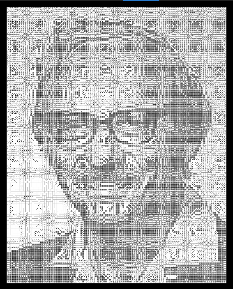
This is not small at all. Although the model is large, it is easy to solve. It only took 11 nodes (most of the work was in the root node). The model is an assignment problem with side constraints [5]. Basically the costs are the difference in gray scale value between the picture and the domino piece for each cell. The constraints are: exactly one domino in each cell and place all dominos. NEOS solves this by processing the picture in Matlab and then solving the model with GAMS/CPLEX. The output PNG file is also notably large: 2.8 MB. Too large to include in this blog. A screen grab looks like:

Screen capture of hi-res image

After zooming in we see indeed the dominos:

Zooming in

With some effort we can recognize part of the frame of the eye glasses here.

References

Thursday, March 26, 2009

Drawing TSP Tour in GAMS

 Can I draw a TSP tour in GAMS?

Yes, use 2D vectors. Here are a few examples: a 29 city problem and a 51 city problem solved as a MIP.


Sunday, March 1, 2009

TSP in OML (MS Solver Foundation)

In theory it is easy to formulate a TSP when the all-different constraint is present. Let x[i] be the ith city visited, an OML-like formulation could look like:

Model[
  Parameters[Integers,N=14],
  Parameters[Sets[Integers],city],
  Parameters[Reals,dist[city,city]],
  Decisions[Integers[0,N-1],x[city]],
  Constraints[
     Unequal[Foreach[{i,city},x[i]]]
  ],
  Goals[
    Minimize[Sum[{i,city},dist[x[i],x[i++1]]]]
  ]
]

This does not work completely. First, bounds can not contain a symbolic constant. Yuck: we need to write [0,13] as bounds:  Decisions[Integers[0,13],x[city]]. The objective has  a few more difficulties. There is no circular lead/lag operator in OML (like the -- or ++ operator in GAMS).  This can be solved by introducing a parameter next[city]. This can be calculated in Excel and imported in the OML model. Furthermore, we cannot use a variable as an index, so dist[x[i],x[next[i]]] is not a valid construct (some languages geared towards solving CSP problems allow this; it adds concise expressiveness to the language that may help the modeler). The error message indicates this is not related to OML per se but rather to solver support. Also it is not allowed to use something like FilteredSum[{j,city},j==x[i],...] (a condition in a FilteredSum cannot depend on a decision variable). The only thing I could think of was:

Minimize[Sum[{i,city},{j,city},{k,city},AsInt[j==x[i]]*AsInt[k==x[next[i]]]*dist[j,k]]]

Note that I used integers as set elements. I started with using data-binding through tables, using set elements {'city0','city1',...,'city13'}. This made the model somewhat more complicated, as x[i] is an integer. So the CSP formulation uses the simpler set {0,1,...,13} allowing us to operate on indices. (Some consider this bad modeling: in GAMS arithmetic on sets is actually discouraged, and needs a function ord()to convert the element — always a string in GAMS — to an integer). Unfortunately I was not able to solve the small 14 city example with the CSP solver using this formulation. (Even after adding City[0]==0 as constraint). To check the input, I also tried a MIP formulation with Gurobi. That solved this small instance just fine.

In the MIP formulation we needed to formulate:

FilteredSum[{i,city},i != 'city0', x['city0',i]]==1

From what I can see this is not possible: a set element not being an integer can not be used in OML. As a workaround I created sets by binding to some dummy parameters:

Sum[{i0,city0},{i,city2},x[i0,i]]==1

where city0 is a set containing only a single element 'city0', and city2 is a set {'city1',...,'city13'}.  The constraint

FilteredSum[{i,city},{j,city},i != j,x[i,j]] <= N

did not work as i and j are not numeric. A workaround could be to have a parameter num[city] which can be calculated in Excel and then imported. Then the condition can read: num[i]!=num[j]. I just used dist[i,j]>0 as condition, as that also can be used to exclude the diagonal (the Excel spreadsheet makes sure all diagonal distances dist[i,i] are zero). A more general approach would be to be able to introduce sparse 2-d sets (like one could do in AMPL and GAMS), but OML has only one dimensional sets as far as I know.

This exercise was really meant to explore the expressiveness of OML. The little model actually shows some interesting issues with OML and some possible workarounds. I do not want to suggest this is a good way to solve TSP's. Obviously these approaches are not suited for large problems. A cutting plane algorithm often is quite effective for slightly larger problems (see this 42 city problem). The excel plugin does not allow us to to implement such an algorithm: an OML model can only contain a single model and has no looping facilities. For the real large problems, you need to look elsewhere, such as Concorde.


Thursday, February 12, 2009

TSP Powerset Formulation

> I'm a PhD student in Portugal and I´m modeling a Vehicle Routing
> Problem. I have some difficulties to modelling this subtour
> elimination constraint (n = number of nodes):

> sum(i in S, sum(j in S, x(i,j))) <= |S|-1
> for every nonempty subset S of {2,3,..,n}


This is the Ford, Fulkerson, Johnson (1954) formulation, based on the power of {2,3,..,n}. This generates a lot of constraints (2^(n-1)), with many not active in the optimal solution. So this approach only works for small problems.

$ontext

  
Burma 14 city problem using power set formulation

  
Erwin Kalvelagen, Amsterdam Optimization

  
References:
       
Gerhard Reinelt, Universitaet Heidelberg, TSPLIB95
       
A.J. Orman & H.P. Williams, A Survey of Different Integer Programming
           
Formulations of the Travelling Salesman Problem

$offtext


$eolcom //

sets
   i
/city1*city14/
   xy
/x,y/
;
alias(i,j);

table coordinates(i,xy) 'coordinates from tsplib'

          
x            y
  
city1  16.47       96.10
  
city2  16.47       94.44
  
city3  20.09       92.54
  
city4  22.39       93.37
  
city5  25.23       97.24
  
city6  22.00       96.05
  
city7  20.47       97.02
  
city8  17.20       96.29
  
city9  16.30       97.38
 
city10  14.05       98.12
 
city11  16.53       97.38
 
city12  21.52       95.59
 
city13  19.41       97.13
 
city14  20.09       94.55
;

*
* form the distance matrix
*
parameter latitude(i), longitude(i), degree(i,xy), minute(i,xy);
degree(i,xy) = trunc(coordinates(i,xy));
minute(i,xy) = coordinates(i,xy) - trunc(coordinates(i,xy));
latitude(i) = pi*(degree(i,
'x')+5.0*minute(i,'x'
)/3.0)/180.0;
longitude(i) = pi*(degree(i,
'y')+5.0*minute(i,'y'
)/3.0)/180.0;


set
nd(i,j);
nd(i,j)$(
not sameas(i,j)) = yes
;


scalar rrr /6378.388/
;
parameter
q1(i,j),q2(i,j),q3(i,j);
q1(nd(i,j)) = cos(longitude(i) - longitude(j));
q2(nd(i,j)) = cos(latitude(i) - latitude(j));
q3(nd(i,j)) = cos(latitude(i) + latitude(j));

parameter c(i,j) 'distance matrix (KM)'
;
c(nd(i,j)) = trunc(RRR * arccos( 0.5*((1.0+q1(i,j))*q2(i,j) - (1.0-q1(i,j))*q3(i,j)) ) + 1.0);
display
c;


*

* form the power set
*
set v(i) 'exclude city 1' /city2*city14/;
abort$(card(i)<>card(v)+1) 'Set v is incorrect'
,i,v;
set n 'subset id (max number of subsets)' /n1*n8192/
;

scalar nsize 'size needed for set n'
;
nsize = 2**
card
(v);
abort$(card(n)<nsize) 'set n is too small'
,nsize;

sets

  base
'used in next set' /no,yes/
  ps0(n,v,base)
/ system.powersetRight/
  ps(n,v)
'power set'
;
ps(n,v) = ps0(n,v,
'yes');


parameter
pscount(n);
pscount(n) =
sum
(ps(n,v),1);

*

* form subsets, exclude subsets with cardinality = 1
*
set nsub(n);
nsub(n)$(pscount(n)>=2) =
yes
;

*

* form ps2(n,i,j) = ps(n,i) and ps(n,j)
* this will simplify the subtour elimination constraint
*
alias(v,vv);
set
ps2(n,i,j);
ps2(nsub(n),nd(v,vv))$(ps(n,v)
and ps(n,vv)) = yes
;

*

* here is the model
*
binary variables x(i,j);
variable z 'objective variable'
;

equations

   obj 
'objective'
   assign1(i)
'assignment problem constraint'
   assign2(j)
'assignment problem constraint'
   subt(n)   
'subtour elimination'
;

obj..   z =e=
sum(nd(i,j), c(i,j)*x(i,j));
assign1(i)..
sum
(nd(i,j), x(i,j)) =e= 1;
assign2(j)..
sum
(nd(i,j), x(i,j)) =e= 1;
subt(nsub(n))..
sum
(ps2(n,i,j),x(i,j)) =L=  pscount(n)-1;

option
optcr=0;
model tsp /all/
;
solve
tsp minimizing z using mip;

Note: the construct system.powerSetRight is a new GAMS feature (24.0, 2013).

This solves quite fast:

--- Starting compilation
--- burma14.gms(122) 9 Mb
--- Starting execution: elapsed 0:00:00.028
--- burma14.gms(120) 21 Mb
--- Generating MIP model tsp
--- burma14.gms(122) 44 Mb
---   8,207 rows  183 columns  320,035 non-zeroes
---   182 discrete-columns
--- Executing CPLEX: elapsed 0:00:00.741

IBM ILOG CPLEX   24.7.3 r58181 Released Jul 11, 2016 WEI x86 64bit/MS Windows
--- GAMS/Cplex licensed for continuous and discrete problems.
Cplex 12.6.3.0

Reading data...
Starting Cplex...
Space for names approximately 0.16 Mb
Use option 'names no' to turn use of names off
Tried aggregator 1 time.
MIP Presolve eliminated 1 rows and 1 columns.
Reduced MIP has 8206 rows, 182 columns, and 319852 nonzeros.
Reduced MIP has 182 binaries, 0 generals, 0 SOSs, and 0 indicators.
Presolve time = 0.28 sec. (95.59 ticks)
Probing time = 0.03 sec. (15.13 ticks)
Tried aggregator 1 time.
Reduced MIP has 8206 rows, 182 columns, and 319852 nonzeros.
Reduced MIP has 182 binaries, 0 generals, 0 SOSs, and 0 indicators.
Presolve time = 0.28 sec. (95.59 ticks)
Probing time = 0.03 sec. (15.13 ticks)
Clique table members: 106.
MIP emphasis: balance optimality and feasibility.
MIP search method: dynamic search.
Parallel mode: none, using 1 thread.
Tried aggregator 1 time.
DUAL formed by presolve
Reduced LP has 182 rows, 8388 columns, and 320034 nonzeros.
Presolve time = 0.08 sec. (27.42 ticks)

Iteration log . . .
Iteration:     1    Objective     =            70.000000
Initializing dual steep norms . . .
Root relaxation solution time = 0.16 sec. (57.42 ticks)

        Nodes                                         Cuts/
   Node  Left     Objective  IInf  Best Integer    Best Bound    ItCnt     Gap

*     0     0      integral     0     3323.0000     3323.0000       45    0.00%
Elapsed time = 1.30 sec. (460.29 ticks, tree = 0.00 MB, solutions = 1)
Found incumbent of value 3323.000000 after 1.30 sec. (460.29 ticks)

Root node processing (before b&c):
  Real time             =    1.30 sec. (460.33 ticks)
Sequential b&c:
  Real time             =    0.00 sec. (0.00 ticks)
                          ------------
Total (root+branch&cut) =    1.30 sec. (460.33 ticks)
MIP status(101): integer optimal solution
Cplex Time: 1.30sec (det. 460.33 ticks)
Fixing integer variables, and solving final LP...
Tried aggregator 1 time.
LP Presolve eliminated 8207 rows and 183 columns.
All rows and columns eliminated.
Presolve time = 0.03 sec. (13.14 ticks)
Fixed MIP status(1): optimal
Cplex Time: 0.03sec (det. 17.45 ticks)

Proven optimal solution.

MIP Solution:         3323.000000    (45 iterations, 0 nodes)
Final Solve:          3323.000000    (0 iterations)

Best possible:        3323.000000
Absolute gap:            0.000000
Relative gap:            0.000000

--- Restarting execution
--- burma14.gms(122) 20 Mb
--- Reading solution for model tsp
--- burma14.gms(122) 20 Mb
*** Status: Normal completion
--- Job burma14.gms Stop 02/23/17 00:47:38 elapsed 0:00:02.719

image

References
  1. burma14.gms: above model
  2. burma14-3.gms: generation of powerset written in GAMS (not using system.PowerSetRight).
  3. burma14-2.gms: formulation from Svestka (J.A. Svestka, A continuous variable representation of the TSP, Math Prog, v15, 1978, pp211-213)
  4. burma14-4.gms: a cutting plane technique

Wednesday, August 6, 2008

How write a TSP model in GAMS

> My TSP model does not work: it has sub-tours

The TSP (Traveling Salesman Problem) is not complete trivial to write as a MIP.
Direct MIP models are only suited for very small problem. For larger models
you need more advanced strategies.

You can see some examples in the model library all written by me: tsp1, tsp2, tsp3, tsp4, tsp42 (the listed author is incorrect: I wrote this model). The last one is actually an algorithm that adds subtour elimination cuts to a relaxation.

For more information see the following papers and posts:


Monday, July 7, 2008

How to call GAMS from Access?

Short Answer: invoke gams.exe using the CreateProcess API call. In a practical application much more is needed:
  1. Create a button so user can launch GAMS
  2. Find the location where GAMS.EXE is located
  3. Create unique directory where scratch files can be read and written
  4. Provide a mechanism to write problem data to a GAMS file
  5. Call GAMS, capture log output and show in window, if needed add an interrupt button to stop the solution process
  6. Provide a mechanism to read solution data from the GAMS run
  7. Presentation of solution
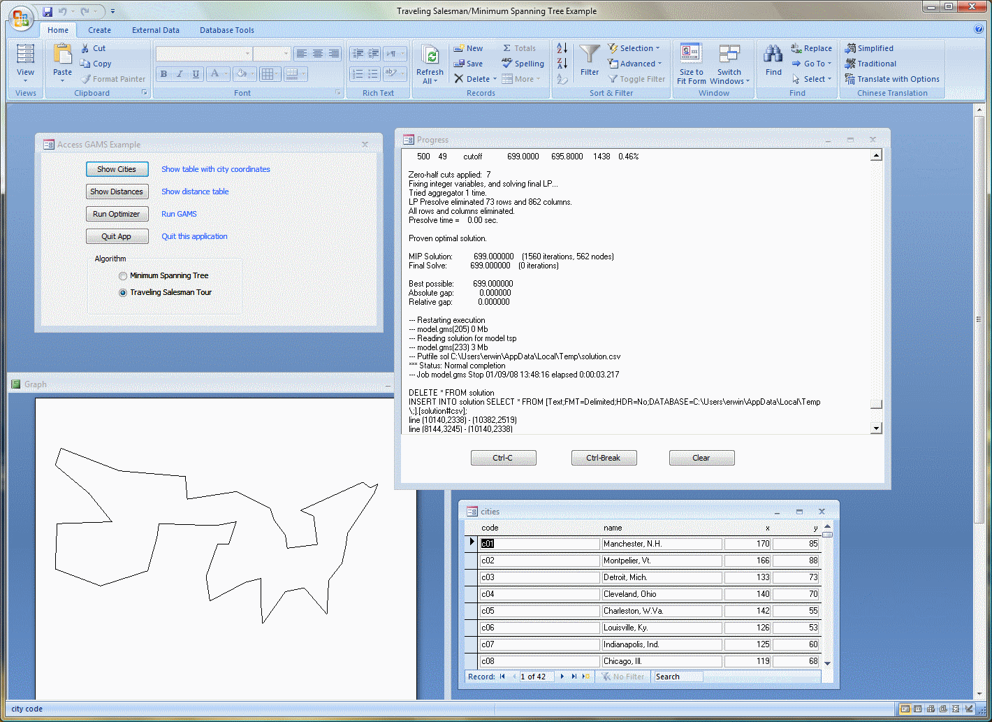
Below is an example: it solves the Traveling Salesman Problem or Minimum Spanning Tree Problem against a 42 US city data set. The TSP is solved using a cutting place algorithm coded in GAMS. All the steps described above are coded in VBA. Click to enlarge.


You'll see four windows inside Access. The first window contains some buttons that allow the user to drive the application. The log window shows any progress by GAMS. It also has some buttons to allow the user to interrupt the solution process. The graph is a simple way to display the solution. The right-lower window shows a data table with city related information (name, coordinates etc.)