Showing posts with label MIQP. Show all posts

Thursday, June 16, 2022

MAX-CUT

The MAX-CUT problem is quite famous [1]. It can be stated as follows:

Given an undirected graph \(G=(V,E)\), split the nodes into two sets. Maximize the number of edges that have one node in each set.

Here is an example using a random sparse graph:

Tuesday, October 27, 2020

Finding a cluster of closest points

Problem statement


From [1]:

Consider \(n=100\) points in an 12 dimensional space. Find \(m=8\) points such that they are as close as possible.


Models


The problem can be stated as a simple MIQP (Mixed Integer Quadratic Programming) model.

 
MINSUM MIQP Model
\[\begin{align} \min & \sum_{i\lt j} \color{darkred}x_i \cdot \color{darkred}x_j \cdot \color{darkblue}{\mathit{dist}}_{i,j} \\ & \sum_i \color{darkred}x_i = \color{darkblue}m \\ & \color{darkred}x_i \in \{0,1\} \end{align}\]


This is a simple model. The main wrinkle is that we want to make sure that we only count each distance once. For this reason, we only consider distances with \(i \lt j\). Of course, we can exploit this also in calculating the distance matrix \( \color{darkblue}{\mathit{dist}}_{i,j}\), and make this a strictly upper-triangular matrix. This saves time and memory.

As the \( \color{darkred}x\) variables are binary, we can easily linearize this problem:


MINSUM MIP Model
\[\begin{align} \min & \sum_{i\lt j} \color{darkred}y_{i,j} \cdot \color{darkblue}{\mathit{dist}}_{i,j} \\ & \color{darkred}y_{i,j} \ge \color{darkred}x_i + \color{darkred}x_j - 1 && \forall i \lt j\\ & \sum_i \color{darkred}x_i = \color{darkblue}m \\ & \color{darkred}x_i \in \{0,1\} \\ &\color{darkred}y_{i,j} \in [0,1] \end{align}\]


The inequality implements the implication \[\color{darkred}x_i= 1 \textbf{ and } \color{darkred}x_j = 1 \Rightarrow \color{darkred}y_{i,j} = 1 \] The variables \(\color{darkred}y_{i,j}\) can be binary or can be relaxed to be continuous between 0 and 1. The MIQP and MIP model should deliver the same results. 

Finally, we can also consider a slightly different problem. Instead of minimizing the sum of the distances between points inside the cluster of the selected points, we can also minimize the maximum distance between points inside the cluster. The (linear) model can look like:

MINMAX MIP Model
\[\begin{align} \min\> & \color{darkred}z \\ & \color{darkred}z \ge \color{darkred}y_{i,j} \cdot \color{darkblue}{\mathit{dist}}_{i,j} && \forall i \lt j \\ & \color{darkred}y_{i,j} \ge \color{darkred}x_i + \color{darkred}x_j - 1 && \forall i \lt j\\ & \sum_i \color{darkred}x_i = \color{darkblue}m \\ & \color{darkred}x_i \in \{0,1\} \\ &\color{darkred}y_{i,j} \in [0,1] \end{align}\]

We re-use our linearization here.

Finally, I also tried a very simple greedy heuristic:
  1. Select the two points that are closest to each other.
  2. Select a new unselected point that is closest to our already selected points.
  3. Repeat step 2 until we have selected 8 points.
We can expect our optimization models to do a bit better than this simplistic approach. 

In our methods here, we did not make any assumptions about the distance metric being used We just needed the distance matrix. This means you can use Euclidean, Manhattan, or other metrics. In addition, you can use some normalization or weighting before calculating the distances. This may be useful if the features have different units. These models also do not change whether one uses low- or high-dimensional data.

There are alternative models one could envision, such as finding the smallest enclosing sphere or box. These methods do not make things simpler and will likely not improve upon our models. 

Small data set


Let's start with selecting \(m=8\) points from  \(n=50\), using random 2d coordinates.


----     10 PARAMETER coord  coordinates

                  x           y

point1        0.172       0.843
point2        0.550       0.301
point3        0.292       0.224
point4        0.350       0.856
point5        0.067       0.500
point6        0.998       0.579
point7        0.991       0.762
point8        0.131       0.640
point9        0.160       0.250
point10       0.669       0.435
point11       0.360       0.351
point12       0.131       0.150
point13       0.589       0.831
point14       0.231       0.666
point15       0.776       0.304
point16       0.110       0.502
point17       0.160       0.872
point18       0.265       0.286
point19       0.594       0.723
point20       0.628       0.464
point21       0.413       0.118
point22       0.314       0.047
point23       0.339       0.182
point24       0.646       0.561
point25       0.770       0.298
point26       0.661       0.756
point27       0.627       0.284
point28       0.086       0.103
point29       0.641       0.545
point30       0.032       0.792
point31       0.073       0.176
point32       0.526       0.750
point33       0.178       0.034
point34       0.585       0.621
point35       0.389       0.359
point36       0.243       0.246
point37       0.131       0.933
point38       0.380       0.783
point39       0.300       0.125
point40       0.749       0.069
point41       0.202       0.005
point42       0.270       0.500
point43       0.151       0.174
point44       0.331       0.317
point45       0.322       0.964
point46       0.994       0.370
point47       0.373       0.772
point48       0.397       0.913
point49       0.120       0.735
point50       0.055       0.576


The MINSUM MIQP and MIP model gives the same solution, but (as expected) the MINMAX model is slightly different. Here are the results with Cplex:

 
          HEURISTIC        MIQP         MIP      MINMAX

point2        1.000
point3                    1.000       1.000       1.000
point9                                            1.000
point10       1.000
point11                   1.000       1.000
point12                                           1.000
point15       1.000
point18                   1.000       1.000       1.000
point20       1.000
point23                   1.000       1.000       1.000
point24       1.000
point25       1.000
point27       1.000
point29       1.000
point35                   1.000       1.000
point36                   1.000       1.000       1.000
point39                   1.000       1.000       1.000
point43                                           1.000
point44                   1.000       1.000
status                  Optimal     Optimal     Optimal
obj                       3.447       3.447       0.210
sum           4.997       3.447       3.447       3.522
max           0.291       0.250       0.250       0.210
time                     33.937       2.125       0.562


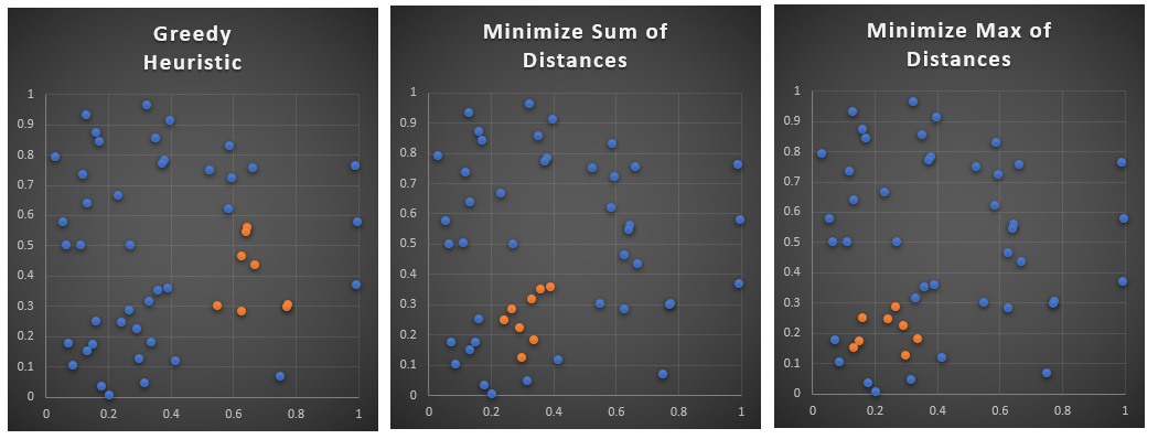
When we plot the results, we see:


Obviously, our optimization models do much better than the heuristic. Two optimization models have quite an overlap in the selected points. To compare the objectives MINSUM and MINMAX we can plot them against each other:


Obviously, our heuristic is not doing that great.

Large data set 


Here we select \(m=8\) points from  \(n=100\), using random 12d coordinates. Using Gurobi on a faster machine we see:


----    112 PARAMETER results  

          HEURISTIC        MIQP         MIP      MINMAX

point5        1.000                               1.000
point8                    1.000       1.000
point17       1.000                               1.000
point19                   1.000       1.000
point24                                           1.000
point35                   1.000       1.000
point38                   1.000       1.000
point39                                           1.000
point42       1.000                               1.000
point43                                           1.000
point45       1.000       1.000       1.000
point51       1.000
point56       1.000
point76       1.000
point81                   1.000       1.000
point89                   1.000       1.000
point94       1.000       1.000       1.000       1.000
point97                                           1.000
status                TimeLimit     Optimal     Optimal
obj                      26.230      26.230       1.147
sum          30.731      26.230      26.230      27.621
max           1.586       1.357       1.357       1.147
time                   1015.984      49.000       9.594
gap%                     23.379


The MINSUM MIQP model hit a time limit of 1000 seconds but actually found the optimal solution. It just did not have the time to prove it. The overlap between the MINSUM models and the MINMAX model is very small (just one shared point). I expected more overlap.

Conclusions


The MINMAX model seems to solve faster than the MINSUM versions. This is a little bit surprising: often these max or min objectives are slower than direct sums. It always pays off to do some experiments with different formulations. Slightly different models can show a large difference in solution times. This is a great example of that.

These models are independent of the dimensionality of the data and the distance metric being used.

References


  1. Given a set of points or vectors, find the set of N points that are closest to each other, https://stackoverflow.com/questions/64542442/given-a-set-of-points-or-vectors-find-the-set-of-n-points-that-are-closest-to-e


Appendix: GAMS code


Some interesting features:
  • There are not that many models where I can use xor operators. Here it is used in the Greedy Heuristic where we want to consider points \(i\) and \(j\) where one of them is in the cluster and one outside. 
  • Of course instead of the condition that x.l(i) xor x.l(j) is nonzero, we also could have required that x.l(i)+x.l(j)=1. I just could not resist the xor.
  • Macros are used to prevent repetitive code in the reporting of results.
  • Acronyms are used in reporting. 


$ontext

 
find cluster of m=8 points closest to each other

 
compare:
      
simple greedy heuristic (HEURISTIC)
      
quadratic model (MIQP)
      
linearized model (MIP)
      
minmax model (MINMAX)

$offtext

set
  c
'coordinates' /x,y/
  i
'points' /point1*point50/
;

scalar m 'number of points to select' /8/;

parameter coord(i,c) 'random coordinates';
coord(i,c) = uniform(0,1);
display coord;

alias(i,j);
set ij(i,j) 'upper triangular structure';
ij(i,j) =
ord(i) < ord(j);

parameter dist(i,j) 'euclidean distances';
dist(ij(i,j)) = sqrt(
sum(c, sqr(coord(i,c)-coord(j,c))));

binary variables x(i) 'selected points';
positive variable y(i,j) 'x(i)*x(j), relaxed to be continuous';
y.up(ij)=1;

variable z 'objective';

equations
    obj1 
'quadratic objective'
    obj2 
'linearized objective'
    obj3 
'minmax objective'
    select
'number of selected points'
    bound 
'implication x(i)=x(j)=1 ==> y(i,j)=1'
;

obj1.. z =e=
sum(ij(i,j), x(i)*x(j)*dist(ij));
obj2.. z =e=
sum(ij, y(ij)*dist(ij));
obj3(ij).. z =g= y(ij)*dist(ij);
select..
sum(i, x(i)) =e= m;
bound(ij(i,j))..  y(i,j) =g= x(i) + x(j) - 1;

model m1 /obj1,select/;
model m2 /obj2,select,bound/;
model m3 /obj3,select,bound/;
option optcr=0,mip=cplex,miqcp=cplex,threads=8;

*------------------------------------------------
* reporting macros
*------------------------------------------------

parameter results(*,*);

set dummy 'ordering for output' /  status, obj, sum, max, time, 'gap%' /;

acronym TimeLimit;
acronym Optimal;

* macros for reporting
$macro sumdist    sum(ij(i,j), x.l(i)*x.l(j)*dist(ij))
$macro maxdist    smax(ij(i,j), x.l(i)*x.l(j)*dist(ij))
$macro report(m,label)  \
    x.l(i) = round(x.l(i));  \
    results(i,label) = x.l(i); \
    results(
'status',label)$(m.solvestat=1) = Optimal; \
    results(
'status',label)$(m.solvestat=3) = TimeLimit; \
    results(
'obj',label) = z.l; \
    results(
'sum',label) = sumdist; \
    results(
'max',label) = maxdist; \
    results(
'time',label) = m.resusd; \
    results(
'gap%',label)$(m.solvestat=3) = 100*abs(m.objest - m.objval)/abs(m.objest);


*------------------------------------------------
* heuristic
*------------------------------------------------


* step 1 : select points 1 and 2 by minimizing distance
scalar dmin,dmin1,dmin2;
dmin =
smin(ij,dist(ij));
loop(ij(i,j)$(dist(ij)=dmin),
   x.l(i)=1;
   x.l(j)=1;
  
break;
);

* add points 3..m, closest to points selected earlier
scalar k;
for(k = 3 to m,
   dmin =
smin(ij(i,j)$(x.l(i) xor x.l(j)), dist(ij));
  
loop(ij(i,j)$(dist(ij)=dmin),
     x.l(i)=1;
     x.l(j)=1;
    
break;
   );
);

results(i,
'HEURISTIC') = x.l(i);
results(
'sum','HEURISTIC') = sumdist;
results(
'max','HEURISTIC') = maxdist;


*------------------------------------------------
* run models m1 through m3
*------------------------------------------------

solve m1 minimizing z using miqcp;
report(m1,
'MIQP')

solve m2 minimizing z using mip;
report(m2,
'MIP')

solve m3 minimizing z using mip;
report(m3,
'MINMAX')

display results;


Monday, August 17, 2020

A variant of the max-sum-subarray problem

In [1] a variant of the max-sum-subarray problem is posed: 

Suppose you have two arrays each containing the same amount of "1"s and "-1"s. Additionally, suppose each "1" in the first array has a corresponding or sibling "1" in the second array. Same for each "-1". The task is to find the optimal subarrays, one in the first array and one in the second, such that their combined sum is the largest (maximal) with the added constraint that an element in one subarray only counts towards the sum if the other subarray contains its sibling.


Example


In [1] the following example is given:


An optimal solution is: select elements 3 through 10 in the first array and elements 5 through 10 in the second array, with a total objective of 8.


Reviewing the max-sum-subarray problem


Let's first review the max-sum-subarray problem [2]. We have data \(a_i\) with both positive and negative numbers. For example:


----      5 SET i  number of elements

i1 ,    i2 ,    i3 ,    i4 ,    i5 ,    i6 ,    i7 ,    i8 ,    i9 ,    i10,    i11,    i12,    i13,    i14,    i15
i16,    i17,    i18,    i19,    i20,    i21,    i22,    i23,    i24,    i25,    i26,    i27,    i28,    i29,    i30
i31,    i32,    i33,    i34,    i35,    i36,    i37,    i38,    i39,    i40,    i41,    i42,    i43,    i44,    i45
i46,    i47,    i48,    i49,    i50


----      5 PARAMETER a  data

i1  -5.280,    i2   8.640,    i3   2.006,    i4  -0.865,    i5  -8.367,    i6   1.227,    i7   2.775,    i8   0.607
i9   5.950,    i10  6.512,    i11  4.469,    i12 -5.984,    i13 -5.207,    i14  0.889,    i15  2.652,    i16  6.418
i17 -5.499,    i18 -9.400,    i19 -6.543,    i20 -6.948,    i21 -1.842,    i22 -6.746,    i23  5.136,    i24  8.559
i25 -6.108,    i26  9.186,    i27 -5.854,    i28  6.325,    i29  6.854,    i30 -8.525,    i31 -8.762,    i32  2.467
i33 -3.522,    i34  3.210,    i35 -2.523,    i36 -2.771,    i37  1.839,    i38 -1.234,    i39  2.501,    i40  4.430
i41  3.220,    i42 -9.646,    i43  6.979,    i44 -4.781,    i45 -6.631,    i46  9.047,    i47  0.211,    i48  6.068
i49 -7.734,    i50  7.059


A standard approach is to introduce two parallel binary variables: \[x_i = \begin{cases} 1 & \text{if data item $a_i$ is selected to be included in the subarray} \\  0 &\text{otherwise}\end{cases}\] and \[\mathit{start}_i = \begin{cases} 1 & \text{when we switch from $x_{i-1}=0$ to $x_{i}=1$} \\  0 &\text{otherwise}\end{cases}\] The integer programming model can look like: 


max-sum-subarray MIP formulation
\[\begin{align}\max\>& \color{darkred} z = \sum_i \color{darkblue}a_i \cdot \color{darkred}x_i \\ & \color{darkred}{\mathit{start}}_i \ge \color{darkred}x_i - \color{darkred}x_{i-1} \\ & \sum_i \color{darkred}{\mathit{start}}_i \le 1 \\ & \color{darkred}x_i \in \{0,1\} \\ & \color{darkred}{\mathit{start}}_i \in \{0,1\} \end{align}\]

We ignored here the else part in the definition of \(\mathit{start}\) and just implement the implication: \[x_{i-1}=0\>{\bf and}\>x_i=1 \Rightarrow \mathit{start}_i=1\] Note that the missing else part leaves variables \(\mathit{start}_i\) unrestricted when we do not switch from 0 to 1. As we only have an upper limit on the number of starts this is no problem. Remarkably, if we want, we can relax the variable \(\mathit{start}_i \) to be continuous between 0 and 1.

When we apply the model on our data set, we see the following results:


----     28 VARIABLE x.L  select a number

i23 1.000,    i24 1.000,    i25 1.000,    i26 1.000,    i27 1.000,    i28 1.000,    i29 1.000


----     28 VARIABLE start.L  start of subarray

i23 1.000


----     28 VARIABLE z.L                   =       24.099  objective

This shows that our optimal sub-array consists of elements 23 through 29.

Original problem


In the original problem, we have two data arrays \(a_i\) and \(b_i\).  In addition, we have a mapping from \(a\) to \(b\). We can encode the original data set as:


----     12 SET i  number of elements

i1 ,    i2 ,    i3 ,    i4 ,    i5 ,    i6 ,    i7 ,    i8 ,    i9 ,    i10


----     12 SET k  array

a,    b


----     12 PARAMETER d  data arrays

           i1          i2          i3          i4          i5          i6          i7          i8          i9

a       1.000      -1.000       1.000       1.000      -1.000      -1.000       1.000      -1.000       1.000
b      -1.000       1.000      -1.000      -1.000       1.000       1.000      -1.000       1.000       1.000

+         i10

a       1.000
b       1.000


----     12 SET map  mapping between a and b

             i1          i2          i3          i4          i5          i6          i7          i8          i9

i1                      YES
i2          YES
i3                                                          YES
i4                                                                      YES
i5                                  YES
i6                                                                                  YES
i7                                                                                                          YES
i8                                              YES
i9                                                                                              YES

  +         i10

i10         YES


The data is organized so we can use the "start" formulation for both arrays in one swoop: \[\begin{align} & \mathit{start}_{k,i} \ge x_{k,i} - x_{k,i-1} && \forall k,i\\ &\sum_i \mathit{start}_{k,i} \le 1 && \forall k \\ & x_{k,i}, \mathit{start}_{k,i} \in \{0,1\} \end{align}\] Adding an index to a data-structure is a trick that can help preventing duplicating equations.

The objective is a bit complicated as only entries are counted when both siblings are selected. So, we can write: \[\sum_{i,j|\mathit{map}(i,j)} (d_{a,i}+d_{b,j})\cdot x_{a,i} \cdot x_{b,j} \] This is a quadratic objective. Some solvers can handle this directly. Note that we don't sum over all \((i,j)\) combinations but only over \((i,j)|\mathit{map}_{i,j}\), which has just 10 elements.

The complete model looks like: 

MIQP formulation
\[\begin{align}\max\>& \color{darkred} z = \sum_{i,j|\color{darkblue}{\mathit{map}}(i,j)} (\color{darkblue}d_{\color{darkgreen}a,i}+\color{darkblue}d_{\color{darkgreen}b,j}) \cdot \color{darkred}x_{\color{darkgreen}a,i}\cdot \color{darkred}x_{\color{darkgreen}b,j} \\ & \color{darkred}{\mathit{start}}_{k,i} \ge \color{darkred}x_{k,i} - \color{darkred}x_{k,i-1} && \forall k,i \\ & \sum_i \color{darkred}{\mathit{start}}_{k,i} \le 1 && \forall k\\ & \color{darkred}x_{k,i} \in \{0,1\} \\ & \color{darkred}{\mathit{start}}_{k,i} \in \{0,1\} \end{align}\]


When we run this, we may get the following solution:


----     39 VARIABLE x.L  select a number

           i1          i2          i3          i4          i5          i6          i7          i8          i9

a       1.000       1.000       1.000       1.000       1.000       1.000       1.000       1.000       1.000
b                                                       1.000       1.000       1.000       1.000       1.000

+         i10

a       1.000
b       1.000


----     39 VARIABLE start.L  start of subarray

           i1          i5

a       1.000
b                   1.000


----     39 VARIABLE z.L                   =        8.000  objective


This is a slightly different solution but with the same objective. One way to get the same solution as described in [1] is to add a second objective: minimize the number of selected numbers (i.e. a sparser solution).  We can do this with a weighted objective: \[\max \sum_{i,j|\mathit{map}(i,j)} (d_{a,i}+d_{b,j})\cdot x_{a,i} \cdot x_{b,j} - \lambda \sum_{k,i} x_{k,i} \] for a small value for \(\lambda\), e.g. \(\lambda = 0.001\). When we run this, we see: 


----     39 VARIABLE x.L  select a number

           i3          i4          i5          i6          i7          i8          i9         i10

a       1.000       1.000       1.000       1.000       1.000       1.000       1.000       1.000
b                               1.000       1.000       1.000       1.000       1.000       1.000


----     39 VARIABLE start.L  start of subarray

           i3          i5

a       1.000
b                   1.000


----     39 VARIABLE z.L                   =        7.986  objective


This corresponds to the solution reported by [1].

Maybe a better approach is to use a lexicographic model. In this case, we don't need a weight \(\lambda\), but instead, solve two problems:

  1. Solve the problem with objective  \[\max\> z_1 = \sum_{i,j|\mathit{map}(i,j)} (d_{a,i}+d_{b,j})\cdot x_{a,i} \cdot x_{b,j} \] 
  2. Record the objective function value of the solution \(z^*_1\).
  3. Add the constraint \[ z^*_1 = \sum_{i,j|\mathit{map}(i,j)} (d_{a,i}+d_{b,j})\cdot x_{a,i} \cdot x_{b,j} \] 
  4. Solve the problem with objective  \[\min\>z_2 = \sum_{k,i} x_{k,i}\]
A disadvantage is that we now have a quadratic constraint in the second problem.


It is not very difficult to linearize this problem. Notice that we only have \(n\) products \(x_{a,i} \cdot x_{b,j}\) as we need only to consider combinations \((i,j)|\mathit{map}_{i,j}\). We can write:


Linear formulation
\[\begin{align}\max\>& \color{darkred} z = \sum_{i,j|\color{darkblue}{\mathit{map}}(i,j)} (\color{darkblue}d_{\color{darkgreen}a,i}+\color{darkblue}d_{\color{darkgreen}b,j}) \cdot \color{darkred}y_{i,j} \\ & \color{darkred}{\mathit{start}}_{k,i} \ge \color{darkred}x_{k,i} - \color{darkred}x_{k,i-1} && \forall k,i \\ & \sum_i \color{darkred}{\mathit{start}}_{k,i} \le 1 && \forall k \\ & \color{darkred}y_{i,j} \le \color{darkred}x_{\color{darkgreen}a,i} && \forall i,j|\color{darkblue}{\mathit{map}}(i,j)\\& \color{darkred}y_{i,j} \le \color{darkred}x_{\color{darkgreen}b,j} && \forall i,j|\color{darkblue}{\mathit{map}}(i,j) \\& \color{darkred}y_{i,j} \ge \color{darkred}x_{\color{darkgreen}a,i}+ \color{darkred}x_{\color{darkgreen}b,j} -1 && \forall i,j|\color{darkblue}{\mathit{map}}(i,j) \\ & \color{darkred}x_{k,i} \in \{0,1\} \\ & \color{darkred}{\mathit{start}}_{k,i} \in \{0,1\} \\ & \color{darkred}y_{i,j} \in \{0,1\} \end{align}\]

A larger data set


Let's create a larger data set:
  • 50 random numbers for \(a\) and \(b\) (not restricted to -1, 1),
  • For simplicity use an identity mapping: \(a_i\) is mapped to \(b_i\)

----     11 SET i  number of elements

i1 ,    i2 ,    i3 ,    i4 ,    i5 ,    i6 ,    i7 ,    i8 ,    i9 ,    i10,    i11,    i12,    i13,    i14,    i15
i16,    i17,    i18,    i19,    i20,    i21,    i22,    i23,    i24,    i25,    i26,    i27,    i28,    i29,    i30
i31,    i32,    i33,    i34,    i35,    i36,    i37,    i38,    i39,    i40,    i41,    i42,    i43,    i44,    i45
i46,    i47,    i48,    i49,    i50


----     11 SET k  array

a,    b


----     11 PARAMETER d  data arrays

           i1          i2          i3          i4          i5          i6          i7          i8          i9

a      -6.565       6.865       1.008      -3.977      -4.156      -5.519      -3.003       7.125      -8.658
b       3.222       5.116       2.549      -4.323      -8.272      -7.950       2.825       0.906      -9.370

+         i10         i11         i12         i13         i14         i15         i16         i17         i18

a       0.004       9.962       1.575       9.823       5.245      -7.386       2.794      -6.810      -4.998
b       5.847      -8.545      -6.487       0.513       5.004      -6.438      -9.317       1.703       2.425

+         i19         i20         i21         i22         i23         i24         i25         i26         i27

a       3.379      -1.293      -2.806      -2.971      -7.370      -6.998       1.782       6.618      -5.384
b      -2.213      -2.826      -5.139      -5.072      -7.390       8.669      -2.401       5.668      -3.999

+         i28         i29         i30         i31         i32         i33         i34         i35         i36

a       3.315       5.517      -3.927      -7.790       0.048      -6.797       7.449      -4.698      -4.284
b      -7.490       4.977      -8.615      -5.960      -9.899      -4.608      -0.003      -6.974      -6.517

+         i37         i38         i39         i40         i41         i42         i43         i44         i45

a       1.879       4.454       2.565      -0.724      -1.734      -7.646      -3.716      -9.069      -3.229
b      -3.387      -3.662      -3.558       9.280       9.872      -2.602      -2.542       5.440      -2.066

+         i46         i47         i48         i49         i50

a      -6.358       2.915       1.215       5.399      -4.044
b       8.262      -7.608       4.710      -8.892       1.526


----     11 SET map  mapping between a and b

             i1          i2          i3          i4          i5          i6          i7          i8          i9

i1          YES
i2                      YES
i3                                  YES
i4                                              YES
i5                                                          YES
i6                                                                      YES
i7                                                                                  YES
i8                                                                                              YES
i9                                                                                                          YES

  +         i10         i11         i12         i13         i14         i15         i16         i17         i18

i10         YES
i11                     YES
i12                                 YES
i13                                             YES
i14                                                         YES
i15                                                                     YES
i16                                                                                 YES
i17                                                                                             YES
i18                                                                                                         YES

  +         i19         i20         i21         i22         i23         i24         i25         i26         i27

i19         YES
i20                     YES
i21                                 YES
i22                                             YES
i23                                                         YES
i24                                                                     YES
i25                                                                                 YES
i26                                                                                             YES
i27                                                                                                         YES

  +         i28         i29         i30         i31         i32         i33         i34         i35         i36

i28         YES
i29                     YES
i30                                 YES
i31                                             YES
i32                                                         YES
i33                                                                     YES
i34                                                                                 YES
i35                                                                                             YES
i36                                                                                                         YES

  +         i37         i38         i39         i40         i41         i42         i43         i44         i45

i37         YES
i38                     YES
i39                                 YES
i40                                             YES
i41                                                         YES
i42                                                                     YES
i43                                                                                 YES
i44                                                                                             YES
i45                                                                                                         YES

  +         i46         i47         i48         i49         i50

i46         YES
i47                     YES
i48                                 YES
i49                                             YES
i50                                                         YES

The solution is found quickly using a good solver. E.g. Cplex needs 0 nodes to solve this to optimality: it finds the optimal solution during preprocessing.


----     44 VARIABLE x.L  select a number

          i10         i11         i12         i13         i14         i15         i16

a       1.000       1.000       1.000       1.000       1.000       1.000       1.000
b       1.000       1.000       1.000       1.000       1.000


----     44 VARIABLE start.L  start of subarray

          i10

a       1.000
b       1.000


----     44 VARIABLE y.L  x('a',i)*x('b',j) for map(i,j)

            i10         i11         i12         i13         i14

i10       1.000
i11                   1.000
i12                               1.000
i13                                           1.000
i14                                                       1.000


----     44 VARIABLE z.L                   =       22.941  objective


We see that \(a\) has more selected numbers than \(b\), The extra ones have no value, but do not incur a cost either. If we use a lexicographic approach, we can find the sparsest optimal solution:


----     55 VARIABLE x.L  select a number

          i10         i11         i12         i13         i14

a       1.000       1.000       1.000       1.000       1.000
b       1.000       1.000       1.000       1.000       1.000


----     55 VARIABLE start.L  start of subarray

          i10

a       1.000
b       1.000


----     55 VARIABLE y.L  x('a',i)*x('b',j) for map(i,j)

            i10         i11         i12         i13         i14

i10       1.000
i11                   1.000
i12                               1.000
i13                                           1.000
i14                                                       1.000


----     55 VARIABLE z.L                   =       22.941  objective
            VARIABLE z2.L                  =       10.000  second level objective: number of elements selected


With the linearized model, we do not generate a quadratic constraint when using the lexicographic algorithm. This removes a complication. The implementation is shown below.

GAMS model


The GAMS implementation of the last model (lexicographic, linearized) can look like:


set
  i
'number of elements' /i1*i50/
  k
'array' /a, b/
;
alias(i,j);

parameter d(k, i) 'data arrays';
d(k,i) = uniform(-10,10);

set map(i,j) 'mapping between a and b';
map(i,i) =
yes;

display i,k,d,map;

binary variables
   x(k,i)
'select a number'
   start(k,i)
'start of subarray'
   y(i,j)
"x('a',i)*x('b',j) for map(i,j)"
;

variable z 'objective: total value';

equations
  obj  
'level 1 obj: total value'
  mul1(i,j) 
'linearization'
  mul2(i,j) 
'linearization'
  mul3(i,j) 
'linearization'
  startbnd(k,i)
'bound on start variable'
  sumstart(k)  
'allow only one start'
;

obj.. z =e=
sum(map(i,j), (d('a',i)+d('b',j))*y(i,j));
mul1(map(i,j)).. y(i,j) =l= x(
'a',i);
mul2(map(i,j)).. y(i,j) =l= x(
'b',j);
mul3(map(i,j)).. y(i,j) =g= x(
'a',i)+x('b',j)-1;
startbnd(k,i).. start(k,i) =g= x(k,i)-x(k,i-1);
sumstart(k)..
sum(i, start(k,i)) =l= 1;

model m /all/;
option optcr=0;
solve m maximizing z using mip;

display x.l, start.l, y.l, z.l;

* fix z to its optimal value
z.fx = z.l;

equation obj2 'second level obj: sparsity';
variable z2 'second level objective: number of elements selected';

obj2.. z2 =e=
sum((k,i), x(k,i));

model m2 /all/;
solve m2 minimizing z2 using mip;
display x.l, start.l, y.l, z.l, z2.l;


More optimization


There is one more optimization we can use.  If the objective coefficient \((d_{a,i}+d_{b,j})\) is positive the model will push \(y_{i,j}\) upwards, so we can drop the constraints \(y_{i,j} \ge x_{a,i}+ x_{b,j} -1\). If on the other hand, \((d_{a,i}+d_{b,j})\) is negative the model will push \(y_{i,j}\) downwards to zero. That means we can drop the constraints: \(y_{i,j} \le x_{b,j}\) and \(y_{i,j} \le x_{b,j}\),  Implementing this can look like: \[\begin{align}& y_{i,j} \le x_{a,i} && \forall i,j|\mathit{map}(i,j), d_{a,i}+d_{b,j} \gt 0\\& y_{i,j} \le x_{b,j} && \forall i,j|\mathit{map}(i,j), d_{a,i}+d_{b,j} \gt 0 \\& y_{i,j} \ge x_{a,i}+ x_{b,j} -1 && \forall i,j|\mathit{map}(i,j), d_{a,i}+d_{b,j} \lt 0\end{align}\] For the special case when \(d_{a,i}+d_{b,j}=0\) we can remove the corresponding \(y_{i,j}\) from the model. For very large data sets this can make a difference.

A second thing to look at is the type of variables \(y\) and \(\mathit{start}\). Instead of being a binary variable, we can relax them to be continuous between 0 and 1.

I did some limited tests, and it looks that we are not really helping Cplex with these tricks. For other solvers, things may be different.  
 

References


Tuesday, August 11, 2020

Largest Rectangular Area in a Histogram

Consider a histogram or bar chart. The problem is to find the largest rectangular area covered by the histogram. A picture will help:

Largest rectangle in a histogram

There are a number of algorithms to attack this problem, some of them very efficient, e.g. \(O(n)\). [1,2]

Here we try to find out if we can formulate this as an optimization model.

A small data set


Here is a small data set. It corresponds to the picture above.


----     13 SET i  bars

i1,    i2,    i3,    i4,    i5,    i6,    i7


----     13 PARAMETER hist  histogram data

i1 6.000,    i2 2.000,    i3 5.000,    i4 4.000,    i5 5.000,    i6 1.000,    i7 6.000


----     13 PARAMETER maxhist              =        6.000  heighest bar


A quadratic model


We start with our central binary variable \[\mathit{select}_i = \begin{cases} 1 & \text{if bar $i$ is selected to be part of the rectangle} \\ 0 & \text{otherwise}\end{cases}\] In addition, we want to know if an unselected bar is left or right of the selected bars. For this we use a binary variable \[\mathit{lr}_i = \begin{cases} 0 & \text{if unselected bar $i$ is to the left of the selected bars} \\ 1& \text{if unselected bar $i$ is to the right of the selected bars} \\ \text{unrestricted} & \text{if $\mathit{select}_i=1$}\end{cases}\] For the above picture, this looks like:


Note that the variable \(\mathit{lr}_i\) can be either 0 or 1 when the corresponding bar is selected.

The variables to describe the rcctangular area are: \(\mathit{start}\), \(\mathit{width}\) and \(\mathit{height}\). 

The following implications can be formed. If bar \(i\) is not selected and to the left, then \(\mathit{start}\gt i\): \[\mathit{select}_i=0  \>{\bf{and}}\> \mathit{lr}_i=0 \Rightarrow  \mathit{start}\ge i+1\] Similarly, if bar \(i\) is not selected and to the right, then \(\mathit{start}+\mathit{width}-1 \lt i\). Formally: \[\mathit{select}_i=0  \>{\bf{and}}\> \mathit{lr}_i=1 \Rightarrow  \mathit{start}+\mathit{width}-1\le i-1\] Furthermore, we also have the implication that limits the height: if bar \(i\) is selected, then \(\mathit{height}\le \mathit{hist}_i\). These implications can be implemented as big-M constraints. Finally, we can link \(\mathit{select}_i\) to the width, by saying: \[\sum_i \mathit{select}_i = \mathit{width}\] The complete model can look like:

Quadratic Model
\[\begin{align}\max&\>\color{darkred}{\mathit{area}}=\color{darkred}{\mathit{width}}\cdot\color{darkred}{\mathit{height}}\\ & \color{darkred}{\mathit{start}} \ge\color{darkblue}i+1-\color{darkblue}n\cdot \color{darkred}{\mathit{select}}_i -\color{darkblue}n\cdot\color{darkred}{\mathit{lr}}_i&& \forall i \\ & \color{darkred}{\mathit{start}}+\color{darkred}{\mathit{width}} \le \color{darkblue} i+\color{darkblue}n\cdot \color{darkred}{\mathit{select}}_i+\color{darkblue}n\cdot (1-\color{darkred}{\mathit{lr}}_i) && \forall i \\ & \sum_i \color{darkred}{\mathit{select}}_i = \color{darkred}{\mathit{width}} \\ & \color{darkred}{\mathit{height}} \le \color{darkblue} {\mathit{hist}}_i + (\color{darkblue}{\mathit{maxhist}} - \color{darkblue} {\mathit{hist}}_i) \cdot (1- \color{darkred}{\mathit{select}}_i) && \forall i \\ & \color{darkred}{\mathit{start}}+\color{darkred}{\mathit{width}}-1 \le \color{darkblue}n \\ & \color{darkred}{\mathit{select}}_i \in \{0,1\} \\ & \color{darkred}{\mathit{lr}}_i \in \{0,1\} \\ & \color{darkred}{\mathit{start}} \in [1,\color{darkblue}n]\\ & \color{darkred}{\mathit{width}} \in [1,\color{darkblue}n]\\ & \color{darkred}{\mathit{height}} \ge 0\\ & \color{darkblue}n = {\bf{card}}(i) \end{align}\]

This is a non-convex MIQP (Mixed Integer Quadratic Programming) model and can be solved with solvers like Baron, Couenne, Antigone, Cplex, and Gurobi. Note that Cplex and Gurobi need a special option to allow these models to be solved: optimalityTarget=3 for Cplex and nonConvex=2 for Gurobi.

Results


After running the model we see:


----     68 VARIABLE select.L  bar is selected

i3 1.000,    i4 1.000,    i5 1.000


----     68 VARIABLE lr.L   unselected bars are left (lr=0) or right (lr=1) of selection

i5 1.000,    i6 1.000,    i7 1.000


----     68 VARIABLE start.L               =        3.000  first selected bar
            VARIABLE width.L               =        3.000  number of selected bars
            VARIABLE height.L              =        4.000  shortest selected bar
            VARIABLE area.L                =       12.000  width*height

Note that zero values are not printed.

A larger data set


To test if this formulation work with a larger data set, I generated some random data:

----     12 SET i  bars

i1  ,    i2  ,    i3  ,    i4  ,    i5  ,    i6  ,    i7  ,    i8  ,    i9  ,    i10 ,    i11 ,    i12 ,    i13 
i14 ,    i15 ,    i16 ,    i17 ,    i18 ,    i19 ,    i20 ,    i21 ,    i22 ,    i23 ,    i24 ,    i25 ,    i26 
i27 ,    i28 ,    i29 ,    i30 ,    i31 ,    i32 ,    i33 ,    i34 ,    i35 ,    i36 ,    i37 ,    i38 ,    i39 
i40 ,    i41 ,    i42 ,    i43 ,    i44 ,    i45 ,    i46 ,    i47 ,    i48 ,    i49 ,    i50 ,    i51 ,    i52 
i53 ,    i54 ,    i55 ,    i56 ,    i57 ,    i58 ,    i59 ,    i60 ,    i61 ,    i62 ,    i63 ,    i64 ,    i65 
i66 ,    i67 ,    i68 ,    i69 ,    i70 ,    i71 ,    i72 ,    i73 ,    i74 ,    i75 ,    i76 ,    i77 ,    i78 
i79 ,    i80 ,    i81 ,    i82 ,    i83 ,    i84 ,    i85 ,    i86 ,    i87 ,    i88 ,    i89 ,    i90 ,    i91 
i92 ,    i93 ,    i94 ,    i95 ,    i96 ,    i97 ,    i98 ,    i99 ,    i100


----     12 PARAMETER hist  histogram data

i1   17.175,    i2   84.327,    i3   55.038,    i4   30.114,    i5   29.221,    i6   22.405,    i7   34.983
i8   85.627,    i9    6.711,    i10  50.021,    i11  99.812,    i12  57.873,    i13  99.113,    i14  76.225
i15  13.069,    i16  63.972,    i17  15.952,    i18  25.008,    i19  66.893,    i20  43.536,    i21  35.970
i22  35.144,    i23  13.149,    i24  15.010,    i25  58.911,    i26  83.089,    i27  23.082,    i28  66.573
i29  77.586,    i30  30.366,    i31  11.049,    i32  50.238,    i33  16.017,    i34  87.246,    i35  26.511
i36  28.581,    i37  59.396,    i38  72.272,    i39  62.825,    i40  46.380,    i41  41.331,    i42  11.770
i43  31.421,    i44   4.655,    i45  33.855,    i46  18.210,    i47  64.573,    i48  56.075,    i49  76.996
i50  29.781,    i51  66.111,    i52  75.582,    i53  62.745,    i54  28.386,    i55   8.642,    i56  10.251
i57  64.125,    i58  54.531,    i59   3.152,    i60  79.236,    i61   7.277,    i62  17.566,    i63  52.563
i64  75.021,    i65  17.812,    i66   3.414,    i67  58.513,    i68  62.123,    i69  38.936,    i70  35.871
i71  24.303,    i72  24.642,    i73  13.050,    i74  93.345,    i75  37.994,    i76  78.340,    i77  30.003
i78  12.548,    i79  74.887,    i80   6.923,    i81  20.202,    i82   0.507,    i83  26.961,    i84  49.985
i85  15.129,    i86  17.417,    i87  33.064,    i88  31.691,    i89  32.209,    i90  96.398,    i91  99.360
i92  36.990,    i93  37.289,    i94  77.198,    i95  39.668,    i96  91.310,    i97  11.958,    i98  73.548
i99   5.542,    i100 57.630


----     12 PARAMETER maxhist              =       99.812  heighest bar


When we solve this we see the following results:


----     67 VARIABLE select.L  selection of bar

i10 1.000,    i11 1.000,    i12 1.000,    i13 1.000,    i14 1.000,    i15 1.000,    i16 1.000,    i17 1.000
i18 1.000,    i19 1.000,    i20 1.000,    i21 1.000,    i22 1.000,    i23 1.000,    i24 1.000,    i25 1.000
i26 1.000,    i27 1.000,    i28 1.000,    i29 1.000,    i30 1.000,    i31 1.000,    i32 1.000,    i33 1.000
i34 1.000,    i35 1.000,    i36 1.000,    i37 1.000,    i38 1.000,    i39 1.000,    i40 1.000,    i41 1.000
i42 1.000,    i43 1.000


----     67 VARIABLE lr.L   unselected bars are left (lr=0) or right (lr=1) of selection

i10  1.000,    i11  1.000,    i13  1.000,    i14  1.000,    i16  1.000,    i19  1.000,    i24  1.000,    i30  1.000
i35  1.000,    i36  1.000,    i37  1.000,    i40  1.000,    i42  1.000,    i44  1.000,    i45  1.000,    i46  1.000
i47  1.000,    i48  1.000,    i49  1.000,    i50  1.000,    i51  1.000,    i52  1.000,    i53  1.000,    i54  1.000
i55  1.000,    i56  1.000,    i57  1.000,    i58  1.000,    i59  1.000,    i60  1.000,    i61  1.000,    i62  1.000
i63  1.000,    i64  1.000,    i65  1.000,    i66  1.000,    i67  1.000,    i68  1.000,    i69  1.000,    i70  1.000
i71  1.000,    i72  1.000,    i73  1.000,    i74  1.000,    i75  1.000,    i76  1.000,    i77  1.000,    i78  1.000
i79  1.000,    i80  1.000,    i81  1.000,    i82  1.000,    i83  1.000,    i84  1.000,    i85  1.000,    i86  1.000
i87  1.000,    i88  1.000,    i89  1.000,    i90  1.000,    i91  1.000,    i92  1.000,    i93  1.000,    i94  1.000
i95  1.000,    i96  1.000,    i97  1.000,    i98  1.000,    i99  1.000,    i100 1.000


----     67 VARIABLE start.L               =       10.000  first selected bar
            VARIABLE width.L               =       34.000  number of selected bars
            VARIABLE height.L              =       11.049  shortest selected bar
            VARIABLE area.L                =      375.674  width*height


Cplex needed 200 seconds for this. We can help Cplex a bit by adding the ordering constraint: \[\mathit{lr}_i \ge \mathit{lr}_{i-1}\] This has a significant impact:


original formulationwith ordering constraint
Objective375.674375.674
Time (s)21024
Nodes95,8306,040
Iterations2,190,751153,255


A simpler model


There is a simpler approach. Instead of a scalar variable \(\mathit{start}\) we use an indexed variable, indicating where we switch from \(\mathit{select}_{i-1}=0\) to \(\mathit{select}_{i}=1\). In our picture:

We want contiguous selected bars, or in other words: only a single start variable can be 1. This can be modeled as \[\begin{align} & \mathit{start}_i \ge \mathit{select}_i-\mathit{select}_{i-1} \\ &\sum_i \mathit{start}_i \le 1 \end{align}\] The first inequality can be interpreted as the following implication: \[\mathit{select}_{i-1}=0 \>{\bf{and}}\>\mathit{select}_{i}=1 \Rightarrow  \mathit{start}_i=1 \] Note, that \(\mathit{start}_i\) is unrestricted in all other cases. This formulation is not uncommon in machine scheduling models where we want to limit the number start-ups. 

With this we can state the following quadratic model:

Quadratic Model
\[\begin{align}\max&\>\color{darkred}{\mathit{area}}=\sum_i \color{darkred}{\mathit{selected}}_i \cdot \color{darkred}{\mathit{height}}\\ & \color{darkred}{\mathit{start}}_i \ge \color{darkred}{\mathit{select}}_i - \color{darkred}{\mathit{select}}_{i-1} && \forall i \\ & \sum_i \color{darkred}{\mathit{start}}_i \le 1 \\ & \color{darkred}{\mathit{select}}_i \in \{0,1\} \\ & \color{darkred}{\mathit{height}} \le \color{darkblue} {\mathit{hist}}_i + (\color{darkblue}{\mathit{maxhist}} - \color{darkblue} {\mathit{hist}}_i) \cdot (1- \color{darkred}{\mathit{select}}_i) && \forall i \\ & \color{darkred}{\mathit{start}}_i \in \{0,1\} \\ & \color{darkred}{\mathit{height}} \ge 0\\ \end{align}\]

This model can be linearized as we multiply a binary variable with a continuous variable [3]. The multiplication \[\begin{align} &y = \delta \cdot x \\ & \delta \in \{0,1\} \\ & x \in [0,U] \end{align}\] can be linearized as: \[\begin{align} & y \le  U \cdot \delta\\ & y \le x \\& y \ge x - U \cdot (1-\delta) \\ &  \delta \in \{0,1\} \\ & x,y \in [0,U] \end{align}\]

After a little bit of algebra (we have the complication that the variable \(\mathit{height}\) can exceed \(\mathit{hist}_i\) for non-selected bars), we arrive at the following linear model:

 
Linear Model
\[\begin{align}\max&\>\color{darkred}{\mathit{area}}=\sum_i \color{darkred}{\mathit{adjHeight}}_i \\ & \color{darkred}{\mathit{start}}_i \ge \color{darkred}{\mathit{select}}_i - \color{darkred}{\mathit{select}}_{i-1} && \forall i \\ & \sum_i \color{darkred}{\mathit{start}}_i \le 1 \\ & \color{darkred}{\mathit{adjHeight}}_i \le \color{darkred}{\mathit{select}}_i \cdot \color{darkblue} {\mathit{hist}}_i && \forall i \\ & \color{darkred}{\mathit{adjHeight}}_i \le \color{darkred}{\mathit{height}} && \forall i \\ & \color{darkred}{\mathit{adjHeight}}_i \ge \color{darkred}{\mathit{height}} - \color{darkblue}{\mathit{maxhist}} \cdot (1- \color{darkred}{\mathit{select}}_i) && \forall i \\ & \color{darkred}{\mathit{select}}_i \in \{0,1\} \\ & \color{darkred}{\mathit{start}}_i \in \{0,1\} \\ & \color{darkred}{\mathit{height}} \ge 0\\ & \color{darkred}{\mathit{adjHeight}}_i \ge 0 \\ \end{align}\]


In this model, we use \[\mathit{adjHeight}_i = \begin{cases} \mathit{height} & \text{if $\mathit{select}_i=1$} \\ 0 & \text{if $\mathit{select}_i=0$}\end{cases}\]

The solution of the small data set for this model looks like: 
 

----     50 VARIABLE select.L  bar is selected

i3 1.000,    i4 1.000,    i5 1.000


----     50 VARIABLE start.L  first selected bar

i3 1.000


----     50 VARIABLE adjHeight.L  adjusted height: heigth*selected(i)

i3 4.000,    i4 4.000,    i5 4.000


----     50 VARIABLE height.L              =        4.000  area height
            VARIABLE area.L                =       12.000  


Of course, we also ran it with the large, random data set. The solution looks like: 
 

----     49 VARIABLE select.L  bar is selected

i10 1.000,    i11 1.000,    i12 1.000,    i13 1.000,    i14 1.000,    i15 1.000,    i16 1.000,    i17 1.000
i18 1.000,    i19 1.000,    i20 1.000,    i21 1.000,    i22 1.000,    i23 1.000,    i24 1.000,    i25 1.000
i26 1.000,    i27 1.000,    i28 1.000,    i29 1.000,    i30 1.000,    i31 1.000,    i32 1.000,    i33 1.000
i34 1.000,    i35 1.000,    i36 1.000,    i37 1.000,    i38 1.000,    i39 1.000,    i40 1.000,    i41 1.000
i42 1.000,    i43 1.000


----     49 VARIABLE start.L  first selected bar

i10 1.000


----     49 VARIABLE adjHeight.L  adjusted height: heigth*selected(i)

i10 11.049,    i11 11.049,    i12 11.049,    i13 11.049,    i14 11.049,    i15 11.049,    i16 11.049,    i17 11.049
i18 11.049,    i19 11.049,    i20 11.049,    i21 11.049,    i22 11.049,    i23 11.049,    i24 11.049,    i25 11.049
i26 11.049,    i27 11.049,    i28 11.049,    i29 11.049,    i30 11.049,    i31 11.049,    i32 11.049,    i33 11.049
i34 11.049,    i35 11.049,    i36 11.049,    i37 11.049,    i38 11.049,    i39 11.049,    i40 11.049,    i41 11.049
i42 11.049,    i43 11.049


----     49 VARIABLE height.L              =       11.049  area height
            VARIABLE area.L                =      375.674  


To compare the performance, let's add the statistics to our table:

MIQP original formulationMIQP with ordering constraintLinear MIP
Objective375.674375.674375.674
Time (s)210240.8
Nodes95,8306,0400
Iterations2,190,751153,255589


Cplex was able to solve the MIP model to optimality during pre-processing, so no branch-and-bound nodes were needed.

Conclusion


The Largest Rectangular Area in a Histogram is easy to explain. Writing down the corresponding optimization model is a  bit more difficult. In addition, different formulations can lead to dramatic differences in performance. Clearly the linearized model is the winner.

References