Yet Another Math Programming Consultant: MAX-CUT

The MAX-CUT problem is quite famous [1]. It can be stated as follows:

Given an undirected graph $G=(V,E)$, split the nodes into two sets. Maximize the number of edges that have one node in each set.

Here is an example using a random sparse graph:

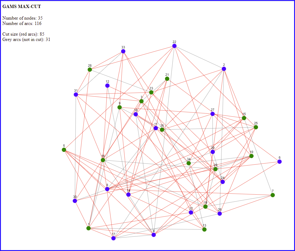MAX CUT, visualization using [2]

Here we colored the two sets of nodes green and blue. We maximize the number of red arcs: they have a green and a blue node. The remaining arcs are grey. We see the optimal solution has a large number of red arcs.

There are some extensions:

The graph can be sparse (as in the figure above): not every pair of nodes has an arc.
We can use weights on the arcs and maximize the weighted sum of red arcs. We can think of the example as using weights $\color{darkblue}w_{i,j}=1$. In this post I assume $\color{darkblue}w_{i,j}\ge 0$.
We can use a directed version: the maximum directed cut.

Max-Cut formulations

To say a node is part of team green or team blue, we just use: \[\color{darkred}x_i = \begin{cases}1 & \text{if node $i$ is a green node}\\ 0 & \text{otherwise}\end{cases}\] I will also indicate the set of selected nodes as $S$. One way to maximum as many red arcs as possible is to use a quadratic formulation:

Unconstrained quadratic model
\[\begin{align}\max&\sum_{(i,j)\in A} \color{darkblue}w_{i,j}\cdot \left(\color{darkred}x_i-\color{darkred}x_j \right)^2 \\ & \color{darkred}x_i\in\{0,1\} \end{align}\]

Here $A$ is the set of arcs. This is non-convex. However, a solver like Cplex will linearize this model automatically for us. We can see this in the log:

Classifier predicts products in MIQP should be linearized.

I.e. Cplex will solve this as a MIP instead of a non-convex MIQP.

We can force Cplex to solve as a quadratic model using the option qtolin=0. After this Cplex will automatically change the problem a bit to make it convex:

Repairing indefinite Q in the objective.

Side note: This repair can be done by adding a multiple of the identity matrix $\lambda I$ to the quadratic Q matrix. This adds essentially terms $\lambda \color{darkred}x_i^2$ to the objective. We can compensate by subtracting the linear terms $\lambda \color{darkred}x_i$. They cancel out, as $\color{darkred}x_i^2=\color{darkred}x_i$ for binary variables.

Instead of using a quadratic objective, we can also use slightly different objectives, such as: \[\max\>\sum_{(i,j)\in A} \color{darkblue}w_{i,j}\cdot \left| \color{darkred}x_i-\color{darkred}x_j \right|\] or \[\max\>\sum_{(i,j)\in A} \color{darkblue}w_{i,j}\cdot \left(\color{darkred}x_i \>{\bf xor }\> \color{darkred}x_j \right)\] Here $\bf xor$ is the "exclusive or" operation, which can be defined by a truth table:

$x$	$y$	$x\>{\bf xor}\>y$
0	0	0
0	1	1
1	0	1
1	1	0

$z =x\>{\bf xor}\>y$ can also be written as a system of linear inequalities: \[\begin{align}&z \le x+y\\ & z \ge x-y \\ & z \ge y-x \\ & z \le 2-x-y\end{align}\] As we are maximizing $z$, we can drop the $\ge$ conditions. Of course, we can also interpret the two included inequalities directly: \[\begin{align} & z \le x+y: && x=y=0 \Rightarrow z=0 \\ & z \le 2-x-y: && x=y=1 \Rightarrow z=0\end{align}\]

So a hand-crafted linear MIP model can look like:

Linear MIP model
\[\begin{align}\max&\sum_{(i,j)\in A} \color{darkblue}w_{i,j}\cdot \color{darkred} e_{i,j}\\ &\color{darkred} e_{i,j} \le\color{darkred}x_i+\color{darkred}x_j && \forall (i,j)\in A\\ & \color{darkred} e_{i,j} \le 2 - \color{darkred}x_i-\color{darkred}x_j && \forall (i,j)\in A \\ & \color{darkred}x_i,\color{darkred}e_{i,j}\in\{0,1\} \end{align}\]

If we want, we can relax $\color{darkred}e_{i,j}$ to be continuous between 0 and 1. Good solvers actually prefer often binary variables in cases like this.

A different MIQP model can be formed by observing that \[\begin{align}\left(\color{darkred}x_i-\color{darkred}x_j \right)^2&=\color{darkred}x_i^2+\color{darkred}x_j^2-2\cdot\color{darkred}x_i\cdot\color{darkred}x_j \\ & =\color{darkred}x_i+\color{darkred}x_j-2\cdot\color{darkred}x_i\cdot\color{darkred}x_j \end{align}\] We used here that $\color{darkred}x^2=\color{darkred}x$ for a binary variable $\color{darkred}x\in \{0,1\}$. With this we can write:

Unconstrained quadratic model v2
\[\begin{align}\max&\sum_{(i,j)\in A} \color{darkblue}w_{i,j}\cdot \left( \color{darkred}x_i + \color{darkred}x_j - 2\cdot\color{darkred}x_i\cdot\color{darkred}x_j \right) \\ & \color{darkred}x_i\in\{0,1\} \end{align}\]

To linearize this, we can use the following set of linear inequalities instead of the binary multiplication $z=x\cdot y$: \[\begin{align}&z \le x\\ & z \le y \\ & z \ge x+y-1 \end{align}\] Because of the nature of the objective, we only need the last constraint: $z \ge x+y-1$. That constraint can be interpreted as $x=y=1 \Rightarrow z=1$.

Linear MIP model v2
\[\begin{align}\max&\sum_{(i,j)\in A} \color{darkblue}w_{i,j}\cdot \left( \color{darkred}x_i + \color{darkred}x_j-2 \cdot \color{darkred} e_{i,j}\right) \\ &\color{darkred} e_{i,j} \ge\color{darkred}x_i+\color{darkred}x_j - 1 && \forall (i,j)\in A \\ & \color{darkred}x_i,\color{darkred}e_{i,j}\in\{0,1\} \end{align}\]

Here are some results of my experiments.

----    200 PARAMETER results  

                  miqp  miqp/nolin         mip   mip/relax   mip/extra     mip/fix   miqp2/fix    mip2/fix

|i|             70.000      70.000      70.000      70.000      70.000      70.000      70.000      70.000
|a|            514.000     514.000     514.000     514.000     514.000     514.000     514.000     514.000
variables       71.000      71.000     585.000     585.000     585.000     585.000      71.000     585.000
 discrete       70.000      70.000     584.000      70.000     584.000     584.000      70.000     584.000
equations        1.000       1.000    1029.000    1029.000    1030.000    1029.000       1.000     515.000
status         Optimal     Optimal     Optimal     Optimal     Optimal     Optimal     Optimal     Optimal
obj            186.232     186.232     186.232     186.232     186.232     186.232     186.232     186.232
time             4.172      25.046      34.250      32.844      35.078      27.328       2.859       2.969
nodes          364.000 1990995.000   32172.000   32172.000   35241.000   22606.000     273.000     310.000
iterations  152218.000 4908384.000 4765712.000 4765712.000 4513440.000 3568752.000   99610.000  108635.000

The columns are:

miqp: MIQP model with default settings, linearized by Cplex. I noticed that Cplex may or may not linearize the same model depending on the data. To be sure linearization is on, use the option qtolin.
miqp/nolin: MIQP without linearization.
mip: linear model.
mip/relax: linear model with $\color{darkred}e$ variables relaxed.
mip/extra: add the constraint: \[\sum_i \color{darkred}x_i \le \sum_i (1-\color{darkred}x_i)\] I.e. fewer selected nodes than unselected ones. This removes some symmetry. Does not seem to help. Note: this constraint can also be stated as \[\sum_i \color{darkred}x_i \le \left\lfloor\frac{\color{darkblue}n}{2}\right\rfloor\] where $\color{darkblue}n$ is the number of nodes.
mip/fix. Of course, another, simpler way to reduce symmetry would be to just fix one node, e.g. $\color{darkred}x_1=1$. This makes some difference.
miqp2/fix. The second quadratic formulation looks a bit faster. This is due to fixing $\color{darkred}x_1=1$. (Both MIQPs are really the same after presolving).
mip2/fix. The linearization of the previous model just has one extra constraint block. With the fixing of node1, this is a really fast MIP.

Small changes in the model can make a difference here.

Running model and generating interactive plot

Max Directed Cut

Here we have a directed graph. We want to maximize the number of arcs $i \rightarrow j$ such that $i \in S$ and $j \notin S$. An example of an optimal solution is:

Here we see that each arc is directed. The curvy arcs indicate there is an arc $i \rightarrow j$ and an arc $j \rightarrow i$. Note that red arcs always start in a blue node (the set $S$) and end in a green node.

This problem can be modeled as:

Unconstrained quadratic model
\[\begin{align}\max&\sum_{(i,j)\in A} \color{darkblue}w_{i,j}\cdot \color{darkred}x_i \cdot \left(1-\color{darkred}x_j \right) \\ & \color{darkred}x_i\in\{0,1\} \end{align}\]

A linearization of this quadratic model can look like:

Linear MIP model
\[\begin{align}\max&\sum_{(i,j)\in A} \color{darkblue}w_{i,j}\cdot \color{darkred}e_{i,j} \\ &\color{darkred}e_{i,j}\le \color{darkred}x_i && \forall (i,j) \in A \\ & \color{darkred}e_{i,j}\le 1-\color{darkred}x_j && \forall (i,j) \in A \\ & \color{darkred}x_i,\color{darkred}e_{i,j}\in\{0,1\} \end{align}\]

If we look at the quadratic objective differently: \[\color{darkred}x_i \cdot \left(1-\color{darkred}x_j \right) = \color{darkred}x_i - \color{darkred}x_i \cdot \color{darkred}x_j\] then we can invent a different linearization:

Linear MIP model v2
\[\begin{align}\max&\sum_{(i,j)\in A} \color{darkblue}w_{i,j}\cdot \left(\color{darkred}x_i-\color{darkred}e_{i,j} \right)\\ &\color{darkred}e_{i,j}\ge \color{darkred}x_i +\color{darkred}x_j-1 && \forall (i,j) \in A \\ & \color{darkred}x_i,\color{darkred}e_{i,j}\in\{0,1\} \end{align}\]

The results are:

----    152 PARAMETER results  

                  miqp  miqp/nolin         mip   mip/relax        mip2

|i|             70.000      70.000      70.000      70.000      70.000
|a|            991.000     991.000     991.000     991.000     991.000
variables       71.000      71.000    1062.000    1062.000    1062.000
 discrete       70.000      70.000    1061.000      70.000    1061.000
equations        1.000       1.000    1983.000    1983.000     992.000
status         Optimal     Optimal     Optimal     Optimal     Optimal
obj            175.650     175.650     175.650     175.650     175.650
time             4.578       1.718       9.109       9.125       4.782
nodes          650.000   62755.000     445.000     445.000     597.000
iterations  221680.000  191587.000  207959.000  207959.000  224287.000

The columns are:

miqp: MIQP formulation. Cplex has linearized this.
miqp/nolin: tell Cplex not to linearize. Cplex will make this problem convex.
mip: direct linearization of the MIQP model.
mip/relax: relax the variables $\color{darkred}e_{i,j}$ to be continuous between 0 and 1.
mip2: alternative linearization.

Interestingly, here we should not linearize, and let Cplex work on the quadratic model.

Warning: Cplex may or may not linearize

As said before: Cplex may or may not linearize a quadratic formulation. Unfortunately, the corresponding messages are deeply buried in the solver log. This can easily lead to wrong conclusions. To illustrate, I use the standard data set g05_60.0 from [3]. I use the objectives: \[\begin{align} (1)&& \max&\sum_{(i,j)\in A} \color{darkblue}w_{i,j}\cdot \left(\color{darkred}x_i-\color{darkred}x_j \right)^2 \\ (2) && \max&\sum_{(i,j)\in A} \color{darkblue}w_{i,j}\cdot \left( \color{darkred}x_i + \color{darkred}x_j - 2\cdot\color{darkred}x_i\cdot\color{darkred}x_j \right) \end{align}\]

The results are:

----    974 PARAMETER results  

              miqp (1)    miqp (2)

|i|             60.000      60.000
|a|            885.000     885.000
variables       61.000      61.000
 discrete       60.000      60.000
equations        1.000       1.000
status         Optimal     Optimal
obj            536.000     536.000
time            13.391     189.094
nodes       986565.000   58361.000
iterations 2492063.000 1.902471E+7

This looks pretty bad for formulation 2. However, studying the solver logs carefully reveals for the first model:

Classifier predicts products in MIQP should not be linearized.

while for the second model:

Classifier predicts products in MIQP should be linearized.

Obviously, letting some machine-learning tool decide what options to use, can lead to surprises. If we tell Cplex not to linearize in both cases, we see:

----    974 PARAMETER results  

              miqp (1)    miqp (2)

|i|             60.000      60.000
|a|            885.000     885.000
variables       61.000      61.000
 discrete       60.000      60.000
equations        1.000       1.000
status         Optimal     Optimal
obj            536.000     536.000
time            13.265      13.219
nodes       986565.000  986565.000
iterations 2492063.000 2492063.000

I.e. in both cases, we solve really the same model (after presolving).

Conclusions

MAX-CUT and MAX-DICUT can be written as relatively simple quadratic or linear models. But there are a few small surprises on the way.
Cplex may reformulate quadratic integer models into linear ones. It decides this on some machine learning model. Downside: it is really unpredictable whether or not this reformulation is applied. You need to study the log carefully to see what Cplex did.
Cplex may also reformulate non-convex quadratic models into convex ones.
This exercise indicates we can actually use quadratic formulations more often than in the past. We used to say: always linearize if possible. This may no longer be the case.
Note that I only ran the models with one single data set. We cannot conclude too much from that.
Solutions are difficult to interpret without visualization tools.

References

Maximum cut, https://en.wikipedia.org/wiki/Maximum_cut
Cytoscape.js, Graph theory (network) library for visualisation and analysis, https://js.cytoscape.org/
Angelika Wiegele, Biq Mac library – a collection of Max-Cut and quadratic 0-1 programming instances of medium size, 2007.

Appendix: GAMS model for undirected max cut problem

$ontext

   MAX CUT (undirected graphs)

   Use random sparse graphs

   Reference:
   http://yetanothermathprogrammingconsultant.blogspot.com/2022/06/max-cut.html

$offtext

* allow all cores to be used
option threads=0;

*---------------------------------------------------------
* undirected graph
*---------------------------------------------------------

set
i 'nodes' /node1*node70/
a(i,i) 'arcs'
;
alias (i,j);

* sparse undirected network
a(i,j)$(ord(i)<ord(j)) = uniform(0,1)<0.2;

parameter w(i,j) 'weights';
w(a) = uniform(0,1);

display$(card(i)<=50) i,a,w;

*------------------------------------------------------------------
* reporting macros
*------------------------------------------------------------------

parameter results(*,*);

acronym Optimal;

* macros for reporting
$macro report(m,label) \
    results('|i|',label) = card(i); \
    results('|a|',label) = card(a); \
    results('variables',label) = m.numvar; \
    results(' discrete',label) = m.numdvar; \
    results('equations',label) = m.numequ; \
    results('status',label)= m.solvestat; \
    results('status',label)$(m.solvestat=1) = Optimal; \
    results('obj',label) = z.l; \
    results('time',label) = m.resusd; \
    results('nodes',label) = m.nodusd; \
    results('iterations',label) = m.iterusd; \
    display results;

*---------------------------------------------------------
* maxcut model 1: unconstrained MIQP
* may be linearized by Cplex
*---------------------------------------------------------

binary variables
   x(i) '1: node is in S, 0: node is not in S'
;

variable z 'objective';

equations
   obj1 'quadratic objective'
;

obj1.. z =e= sum(a(i,j),w(i,j)*sqr(x(i)-x(j)));

model maxcut1 /obj1/;
option miqcp=cplex;
solve maxcut1 maximizing z using miqcp;

parameter ecut(i,j) 'maximum cut';
ecut(a(i,j)) = w(i,j)*sqr(x.l(i)-x.l(j));

option x:0;
display x.l,ecut,z.l;

report(maxcut1,"miqp")

*---------------------------------------------------------
* as maxcut model 1 but prevent automatic linearization
*---------------------------------------------------------

$onecho > cplex.opt
qtolin 0
$offecho

maxcut1.optfile=1;
solve maxcut1 maximizing z using miqcp;
report(maxcut1,"miqp/nolin")

*---------------------------------------------------------
* maxcut model 2:
*---------------------------------------------------------

binary variables e(i,i) 'arc e has one node in S and one not in S';

equations
   obj2     'linear objective'
   e1(i,j) 'implication: x(i)=x(j)=0 ==> e(i,j)=0'
   e2(i,j) 'implication: x(i)=x(j)=1 ==> e(i,j)=0'
;

obj2.. z =e= sum(a,w(a)*e(a));
e1(a(i,j)).. e(i,j) =l= x(i)+x(j);
e2(a(i,j)).. e(i,j) =l= 2-x(i)-x(j);

model maxcut2 /obj2,e1,e2/;
solve maxcut2 maximizing z using mip;

option e:0;
display x.l,e.l,z.l;

report(maxcut2,"mip")

*---------------------------------------------------------
* as model 2 but relax variables e(i,j)
*---------------------------------------------------------

e.prior(a) = +inf;
solve maxcut2 maximizing z using mip;
report(maxcut2,"mip/relax")
e.prior(a) = 1;

*---------------------------------------------------------
* as model 2 but add: sum(x) <= floor(n/2)
* same as sum(x)<=sum(1-x)
*---------------------------------------------------------

equation extra;
extra.. sum(i, x(i)) =l= sum(i, 1-x(i));
* extra.. sum(i,x(i)) =l= floor(card(i)/2);

model maxcut2e /maxcut2,extra/;
solve maxcut2e maximizing z using mip;

report(maxcut2e,"mip/extra")

*---------------------------------------------------------
* as model 2 but fix node1 to 1
*---------------------------------------------------------

x.fx('node1') = 1;
solve maxcut2 maximizing z using mip;
display x.l,e.l,z.l;

report(maxcut2,"mip/fix")

* to unfix do:
*x.lo('node1') = 0;
*x.up('node1') = 1;
* let's keep it fixed

*---------------------------------------------------------
* model 3: different quadratic formulation
*---------------------------------------------------------

equations
   obj3 'model 3 quadratic objective'
;

obj3.. z =e= sum(a(i,j),w(i,j)*(x(i)+x(j)-2*x(i)*x(j)));

model maxcut3 /obj3/;
solve maxcut3 maximizing z using miqcp;

display x.l,z.l;

report(maxcut3,"miqp2/fix")

*---------------------------------------------------------
* model 4: linearization of model 3
*---------------------------------------------------------

equations
   obj4 'linearization of obj3'
   e4(i,j) 'x(i)=x(j)=1 => e(i,j)=1'
;

obj4.. z =e= sum(a(i,j),w(i,j)*(x(i)+x(j)-2*e(i,j)));
e4(a(i,j)).. e(i,j) =g= x(i)+x(j)-1;

model maxcut4 /obj4,e4/;
solve maxcut4 maximizing z using mip;

ecut(a(i,j)) = w(i,j)*sqr(x.l(i)-x.l(j));

display x.l,e.l,z.l;

report(maxcut4,"mip2/fix")

Appendix: GAMS model for max directed cut

$ontext

   MAX DIRECTED CUT (MAX CUT for directed graphs)

   Use random sparse graphs

   Reference:
   http://yetanothermathprogrammingconsultant.blogspot.com/2022/06/max-cut.html

$offtext

* allow all cores to be used, and look for optimal solution
option threads=0,optcr=0;

*---------------------------------------------------------
* directed graph
*---------------------------------------------------------

set
i 'nodes' /node1*node70/
a(i,i) 'arcs'
;
alias (i,j);

* sparse graph
a(i,j) = uniform(0,1)<0.2;

parameter w(i,j) 'weights';
w(a) = uniform(0,1);

display$(card(i)<=50) i,a,w;

*------------------------------------------------------------------
* reporting macros
*------------------------------------------------------------------

parameter results(*,*);

acronym Optimal;

* macros for reporting
$macro report(m,label) \
    results('|i|',label) = card(i); \
    results('|a|',label) = card(a); \
    results('variables',label) = m.numvar; \
    results(' discrete',label) = m.numdvar; \
    results('equations',label) = m.numequ; \
    results('status',label)= m.solvestat; \
    results('status',label)$(m.solvestat=1) = Optimal; \
    results('obj',label) = z.l; \
    results('time',label) = m.resusd; \
    results('nodes',label) = m.nodusd; \
    results('iterations',label) = m.iterusd; \
    display results;

*---------------------------------------------------------
* maxcut model 1
*---------------------------------------------------------

binary variables
   x(i) 'node is in set S'
;

variable z 'objective';

equations
   obj1 'Quadratic objective'
;

obj1.. z =e= sum(a(i,j),w(i,j)*x(i)*(1-x(j)));

model maxcut1 /obj1/;
option miqcp=cplex;
solve maxcut1 maximizing z using miqcp;

parameter ecut(i,j) 'maximum cut';
ecut(a(i,j)) = x.l(i)*(1-x.l(j));

option x:0,ecut:0;
display x.l,ecut,z.l;

report(maxcut1,"miqp")

*---------------------------------------------------------
* as maxcut model 2 but prevent automatic linearlization
*---------------------------------------------------------

$onecho > cplex.opt
qtolin 0
$offecho

maxcut1.optfile=1;
solve maxcut1 maximizing z using miqcp;
report(maxcut1,"miqp/nolin")

*---------------------------------------------------------
* maxcut model 2
*---------------------------------------------------------

binary variables e(i,i) 'arc e is part of cut';

equations
   obj2    'linear objective'
   e1(i,j) 'x(i)=0 ==> e(i,j)=0'
   e2(i,j) 'x(j)=1 ==> e(i,j)=0'
;

obj2.. z =e= sum(a,w(a)*e(a));
e1(a(i,j)).. e(i,j)=l=x(i);
e2(a(i,j)).. e(i,j)=l=1-x(j);

model maxcut2 /obj2,e1,e2/;
solve maxcut2 maximizing z using mip;

option e:0;
display x.l,e.l,z.l;

report(maxcut2,"mip")

*---------------------------------------------------------
* as maxcut model 2 but relax e to be continuous
*---------------------------------------------------------

e.prior(a) = +inf;
solve maxcut2 maximizing z using mip;
report(maxcut2,"mip/relax")
e.prior(a) = 1;

*---------------------------------------------------------
* model 3: linearize x(i)*x(j)
*---------------------------------------------------------

equations
   obj3     'alternative linearization'
   e3(i,j) 'x(i)=x(j)=1 ==> e(i,j)=1'
;

obj3.. z =e= sum(a(i,j),w(i,j)*(x(i)-e(i,j)));
e3(a(i,j)).. e(i,j) =g= x(i)+x(j)-1;
model maxcut3 /obj3,e3/;
solve maxcut3 maximizing z using mip;

display x.l,e.l,z.l;

report(maxcut3,"mip2")

Yet Another Math Programming Consultant

Thursday, June 16, 2022

MAX-CUT