Experiments with Hostile Brothers nonconvex NLP model

In this post, let's do some experiments with the "hostile brothers problem." We have a plot of land. In my test models \([L,U]\times [L,U]\) with \(L=0\), \(U=100\)). We want to place \(n\) brothers on this plot. As they don't get along, we want to spread them out by maximizing the distance between neighbors. In modeling terms, we create a maximin model that maximizes the minimum distance between any two brothers. This yields some non-convex problems, so I'll make the problem small: we just have \(n=10\) brothers. This is a very small, but awe-inspiring problem.

Largest empty shapes

Finding the largest empty shapes

This post is about finding empty regions (square, rectangle, or circle) in a (large) collection of given points. These are interesting little optimization problems.

Data

I generated \(n=100\) data points \((x_i,y_i), i=1,\dots,n\) drawn from a uniform distribution \[\begin{align}&x_i \sim U(0,10) \\ & y_i \sim U(0,10)\end{align} \] 

It is always a good idea to have a careful look at the data. I.e., print and plot it (for very large datasets, print or plot a subset), and collect some elementary statistics (min, max, average, etc.). In practical modeling, it is surprising how many problems arise from simple data errors.  

Revisiting a crazy global NLP problem

Minimum encompassing triangle

This looks like a simple problem. Given \(n\) 2d points, find the smallest encompassing triangle. I follow the formulation from [1]. This post is self-contained, so you don't have to go back to [1]. The main contribution here is how one could work around the performance issues of the original formulation. 

Summary

The problem can be formulated as a nonconvex quadratic problem. However, this leads to models that are very difficult for global NLP solvers: global optimality can not be proven in reasonable time, even for very small data sets. One possible way to attack the problem is to use a different measure for size of the triangle: circumference instead of the more obvious area of a triangle. Although there are explicit algorithms for this problem [3,4], here we are trying to use an optimization model.

Circle Packing and HTML reporting

Little example. Here, we try to pack \(n\) circles with a given radius \(r_i\) into a larger disc with an unknown radius \(R\). The goal is to minimize \(R\). The underlying model is simple: 

Packing of Circles
\[\begin{align} \min\> & \color{darkred}R \\ & \sum_c \left(\color{darkred}p_{i,c}-\color{darkred}p_{j,c}\right)^2 \ge \left(\color{darkblue}r_i+\color{darkblue}r_j\right)^2 & \forall i\lt j \\ & \sum_c \color{darkred}p_{i,c}^2 \le \left(\color{darkred}R-\color{darkblue}r_i\right)^2 & \forall i \\ & \color{darkred}R \ge 0\\ & c \in \{x,y\} \\ \end{align}\]

Another very small but very difficult global NLP model

The goal of this exercise is to fill a square area \([0,250]\times[0,100]\) with 25 circles. The model can choose the \(x\) and \(y\) coordinates of the center of each circle and the radius. So we have as variables \(\color{darkred}x_i\), \(\color{darkred}y_i\), and \(\color{darkred}r_i\). The circles placed inside the area should not overlap. The objective is to maximize the total area covered. 

A solution is:

Small non-convex MINLP: Pyomo vs GAMS

 In [1], the following Pyomo model (Python fragment) is presented:

model.x = Var(name="Number of batches", domain=NonNegativeIntegers, initialize=10)                    
model.a = Var(name="Batch Size", domain=NonNegativeIntegers, bounds=(5,20))

# Objective function
def total_production(model):
    return model.x * model.a
model.total_production = Objective(rule=total_production, sense=minimize)

# Constraints
# Minimum production of the two output products
def first_material_constraint_rule(model):
    return sum(0.2 * model.a * i for i in range(1, value(model.x)+1)) >= 70
model.first_material_constraint = Constraint(rule=first_material_constraint_rule)

def second_material_constraint_rule(model):
    return sum(0.8 * model.a * i for i in range(1, value(model.x)+1)) >= 90
model.second_material_constraint = Constraint(rule=second_material_constraint_rule)

# At least one production run
def min_production_rule(model):
    return model.x >= 1
model.min_production = Constraint(rule=min_production_rule)

Tiny non-convex quadratic model brings solvers to their knees

Here is a very small geometric problem:

Given \(n\) points in 2d space, find the smallest triangle that contains all these points.

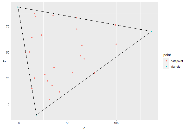Find the smallest triangle containing all points.

This looks like a simple problem. Somewhat to my surprise, my attempt here does not bear that out.

Maximizing Standard Deviation

In [1] a question was posed: how to maximize the standard deviation of a vector \(\color{darkred}x_i\), subject to side constraints using an LP/MIP formulation?

The standard deviation is usually defined as: \[\mathbf{sd}(x) = \sqrt{\frac{1}{n-1}\sum_i \left(x_i-\mu\right)^2}\] where \[\mu = \frac{\sum_i x_i}{n}\] and \(n\) is the number of elements in \(x\).

A multi-objective nonlinear integer programming problem

Picture of the efficient points

In [1], a small multi-objective non-convex MINLP problem is stated:

Let's see how one could approach a problem like this.

Total Least Squares: nonconvex optimization

Total Least Squares (TLS) is an alternative for OLS (Ordinary Least Squares). It is a form of orthogonal regression and also deals with the problem of EIV (Errors-in-Variables). 

The standard OLS model is \[\color{darkblue}y = \color{darkblue}X\color{darkred}\beta + \color{darkred}\varepsilon\] where we minimize the sum-of-squares of the residuals \[\min ||\color{darkred}\varepsilon||_2^2\] We can interpret \(\color{darkred}\varepsilon\) as the error in \(\color{darkblue}y\).

In TLS, we also allow for errors in \(\color{darkblue}X\). The model becomes \[\color{darkblue}y+\color{darkred}\varepsilon=(\color{darkblue}X+\color{darkred}E)\color{darkred}\beta\] Note that we made a sign change in \(\color{darkred}\varepsilon\). This is pure aesthetics: to make the equation more symmetric looking. The objective is specified as \[\min \> ||\left(\color{darkred}\varepsilon \> \color{darkred}E\right)||_F\] i.e. the Frobenius norm of the matrix formed by \(\color{darkred}\varepsilon\) and \(\color{darkred}E\). The Frobenius norm is just \[||A||_F=\sqrt{\sum_{i,j}a_{i,j}^2}\] We can drop the square root from the objective (the solution will remain the same, but we got rid of a non-linear function with a possible problem near zero: the gradient is not defined there). The remaining problem is a non-convex quadratic problem which can be solved with global MINLP solvers such as Baron or with a global quadratic solver like Gurobi.

Maximum Correlation, Global MINLP vs GA

In [1], the following question is posed:

Suppose we have data like:

worker weight height weight2 height2
1      120    60     125     60
2      152    55     156     66
3      222    55     100     20

We can for each case pick (weight,height) or (weight2,height2).  The problem is to pick one of these observations for each row such that the correlation between weight and height is maximized.

Data 

First, let's invent some data that we can use for some experiments. 

----     27 PARAMETER data  

        height1     weight1     height2     weight2

i1    67.433285  168.262871   67.445523  163.692389
i2    70.638374  174.437750   68.649190  160.084811
i3    71.317794  159.909672   69.503911  164.720010
i4    59.850261  145.704159   61.175728  142.708300
i5    65.341938  155.586984   68.483909  165.564991
i6    64.142009  154.335001   68.568683  166.169507
i7    67.030368  158.768813   65.780803  153.721717
i8    73.672863  175.126951   73.236515  164.704340
i9    65.203516  157.593587   63.279277  149.784500
i10   69.001848  160.063428   68.786656  162.278007
i11   64.455422  159.039195   63.930208  152.827710
i12   70.719334  164.885704   69.666096  157.356595
i13   65.688428  151.223468   63.614565  150.071072
i14   66.569252  160.978671   70.533320  160.722483
i15   78.417676  172.298652   80.070076  172.695207
i16   65.396154  158.234709   67.404942  158.310596
i17   62.504967  150.899428   61.000439  154.094647
i18   62.122630  150.024298   63.634554  153.644324
i19   70.598400  165.086523   72.999194  166.771223
i20   74.935107  170.820610   76.622182  169.013550
i21   63.233956  154.331546   60.372876  149.152520
i22   72.550105  173.961915   76.748649  167.462369
i23   74.086553  168.190867   75.433331  171.773607
i24   65.379648  163.577697   65.717553  160.134888
i25   64.003038  155.357607   67.301426  158.713710

The optimal solution that has the highest correlation coefficient between height and weight is:

----     92 PARAMETER result  optimal selected observations

        height1     weight1     height2     weight2

i1                            67.445523  163.692389
i2                            68.649190  160.084811
i3                            69.503911  164.720010
i4    59.850261  145.704159
i5    65.341938  155.586984
i6    64.142009  154.335001
i7    67.030368  158.768813
i8                            73.236515  164.704340
i9                            63.279277  149.784500
i10   69.001848  160.063428
i11                           63.930208  152.827710
i12   70.719334  164.885704
i13                           63.614565  150.071072
i14                           70.533320  160.722483
i15   78.417676  172.298652
i16                           67.404942  158.310596
i17   62.504967  150.899428
i18   62.122630  150.024298
i19                           72.999194  166.771223
i20   74.935107  170.820610
i21                           60.372876  149.152520
i22                           76.748649  167.462369
i23                           75.433331  171.773607
i24                           65.717553  160.134888
i25                           67.301426  158.713710

The impact of being allowed to choose between observations (height1,weight1) and (height2,weight2) is significant:

 

Correlation coefficients
height1-weight1	0.868691
height2-weight2	0.894532
optimal	0.956452

Below we shall see how we arrive at this conclusion.

MINLP Model

A high-level Mixed-Integer Non-Linear Programming model is simply:

MINLP Model

\[ \begin{align}\max\> &\mathbf{cor}(\color{darkred}h,\color{darkred}w) \\ & \color{darkred}h_i = \color{darkblue}{\mathit{height1}}_i\cdot(1-\color{darkred}x_i)+ \color{darkblue}{\mathit{height2}}_i\cdot\color{darkred}x_i\\ & \color{darkred}w_i = \color{darkblue}{\mathit{weight1}}_i\cdot(1-\color{darkred}x_i)+ \color{darkblue}{\mathit{weight2}}_i\cdot\color{darkred}x_i \\ & \color{darkred}x_i \in \{0,1\} \end{align}\]

Here \(\mathbf{cor}(h,w)\) indicates the (Pearson) correlation between vectors \(h\) and \(w\). It is noted that height and weight are positively correlated, so maximizing makes sense.  Of course, GAMS does not know about correlations, so we implement this model as:

 

Implementation of MINLP Model

\[ \begin{align}\max\> & \color{darkred}z = \frac{\displaystyle\sum_i (\color{darkred}h_i-\bar{\color{darkred}h})(\color{darkred}w_i-\bar{\color{darkred}w})}{\sqrt{\displaystyle\sum_i(\color{darkred}h_i-\bar{\color{darkred}h})^2}\cdot \sqrt{\displaystyle\sum_i(\color{darkred}w_i-\bar{\color{darkred}w})^2}} \\ & \color{darkred}h_i = \color{darkblue}{\mathit{height1}}_i\cdot(1-\color{darkred}x_i)+ \color{darkblue}{\mathit{height2}}_i\cdot\color{darkred}x_i \\ & \color{darkred}w_i = \color{darkblue}{\mathit{weight1}}_i\cdot(1-\color{darkred}x_i)+ \color{darkblue}{\mathit{weight2}}_i\cdot\color{darkred}x_i \\ & \bar{\color{darkred}h} = \frac{1}{n}\displaystyle\sum_i \color{darkred}h_i \\ & \bar{\color{darkred}w} = \frac{1}{n}\displaystyle\sum_i \color{darkred}w_i \\ & \color{darkred}x_i \in \{0,1\} \end{align}\]

We need to watch when using divisions. I typically like to reformulate divisions by multiplications: \[\begin{align} \max \>&  \color{darkred}z\\ &\color{darkred}z\cdot \sqrt{\displaystyle\sum_i(\color{darkred}h_i-\bar{\color{darkred}h})^2}\cdot \sqrt{\displaystyle\sum_i(\color{darkred}w_i-\bar{\color{darkred}w})^2} = \displaystyle\sum_i (\color{darkred}h_i-\bar{\color{darkred}h})(\color{darkred}w_i-\bar{\color{darkred}w})\end{align}\]

The advantage of this formulation is in the protection against division by zero. A disadvantage is that non-linearities are moved to the constraints. Many NLP solvers are happier when constraints are linear, and only the objective is non-linear. My answer: experiment with formulations.

When we solve this model with GAMS/Baron, we see:

----     79 VARIABLE x.L  select 1 or 2

i1  1.000000,    i2  1.000000,    i3  1.000000,    i8  1.000000,    i9  1.000000,    i11 1.000000,    i13 1.000000
i14 1.000000,    i16 1.000000,    i19 1.000000,    i21 1.000000,    i22 1.000000,    i23 1.000000,    i24 1.000000
i25 1.000000


----     79 VARIABLE z.L                   =     0.956452  objective

----     83 PARAMETER corr  

all1    0.868691,    all2    0.894532,    optimal 0.956452

The parameter corr shows different correlations:

• When all \(x_i=0\), that is when we compare height1 vs weight1.
• When all \(x_i=1\), so we compare  height2 vs weight2.
• When using an optimal solution for \(x\). 

Nonconvex MIQCP

 

Gurobi can solve non-convex quadratic models quite efficiently. To try this out, I reformulated the MINLP model into a Mixed-Integer Quadratically-Constrained Programming model. We need to add some variables and constraints to make this happen. 

Non-convex MIQCP Model

\[ \begin{align}\max\> & \color{darkred}z\\ & \color{darkred}z\cdot \color{darkred}{\mathit{denom}} = \sum_i (\color{darkred}h_i-\bar{\color{darkred}h})(\color{darkred}w_i-\bar{\color{darkred}w})\\ & \color{darkred}s^2_h = \sum_i(\color{darkred}h_i-\bar{\color{darkred}h})^2 \\ & \color{darkred}s^2_w = \sum_i(\color{darkred}w_i-\bar{\color{darkred}w})^2 \\ & \color{darkred}{\mathit{denom}} = \color{darkred}s_h \cdot \color{darkred}s_w\\ & \color{darkred}h_i = \color{darkblue}{\mathit{height1}}_i\cdot(1-\color{darkred}x_i)+ \color{darkblue}{\mathit{height2}}_i\cdot\color{darkred}x_i \\ & \color{darkred}w_i = \color{darkblue}{\mathit{weight1}}_i\cdot(1-\color{darkred}x_i)+ \color{darkblue}{\mathit{weight2}}_i\cdot\color{darkred}x_i \\ & \bar{\color{darkred}h} = \frac{1}{\color{darkblue}n}\displaystyle\sum_i \color{darkred}h_i \\ & \bar{\color{darkred}w} = \frac{1}{\color{darkblue}n}\displaystyle\sum_i \color{darkred}w_i \\ & \color{darkred}x_i \in \{0,1\} \\ & \color{darkred}s_h, \color{darkred}s_w \ge 0 \end{align}\]

The final model is still quite small, but I encountered severe problems:

Gurobi Optimizer version 9.0.1 build v9.0.1rc0 (win64)
Optimize a model with 52 rows, 81 columns and 152 nonzeros
Model fingerprint: 0xc1d6aa23
Model has 4 quadratic constraints
Variable types: 56 continuous, 25 integer (25 binary)
Coefficient statistics:
  Matrix range     [1e-02, 1e+01]
  QMatrix range    [1e+00, 2e+01]
  QLMatrix range   [1e+00, 1e+00]
  Objective range  [1e+00, 1e+00]
  Bounds range     [1e+00, 2e+02]
  RHS range        [6e+01, 2e+02]
Presolve removed 50 rows and 50 columns
Presolve time: 0.02s
Presolved: 179 rows, 88 columns, 637 nonzeros
Presolved model has 7 bilinear constraint(s)
Variable types: 63 continuous, 25 integer (25 binary)

Root relaxation: unbounded, 0 iterations, 0.00 seconds

    Nodes    |    Current Node    |     Objective Bounds      |     Work
 Expl Unexpl |  Obj  Depth IntInf | Incumbent    BestBd   Gap | It/Node Time

     0     2  postponed    0               -          -      -     -    0s
 50873 43644  postponed  872               -          -      -   0.0    5s
 124683 118126  postponed  805               -          -      -   0.0   10s
 196009 189074  postponed 1409               -          -      -   0.0   15s
 268890 261269  postponed 1771               -          -      -   0.0   20s
 341602 333841  postponed 2653               -          -      -   0.0   25s
 416698 408963  postponed 2652               -          -      -   0.0   30s
 491794 484945  postponed 2764               -          -      -   0.0   35s
 566890 559155  postponed 3533               -          -      -   0.0   40s
 641986 634407  postponed 4413               -          -      -   0.0   45s
 717082 709397  postponed 5294               -          -      -   0.0   50s
 792178 784445  postponed 5296               -          -      -   0.0   55s
 867274 859517  postponed 5295               -          -      -   0.0   60s
 942370 934643  postponed 6177               -          -      -   0.0   65s
 1016274 1009505  postponed 6177               -          -      -   0.0   70s
 1091370 1083743  postponed 7052               -          -      -   0.0   75s
 1166466 1158805  postponed 7939               -          -      -   0.0   80s
 1241562 1233913  postponed 7938               -          -      -   0.0   85s
 1316658 1308953  postponed 7939               -          -      -   0.0   90s
 1391754 1384013  postponed 8820               -          -      -   0.0   95s
 1465658 1457969  postponed 8820               -          -      -   0.0  100s
. . .

This goes on like this for much longer: no feasible solution is found. This looks very bad. Very strange, because this MIQCP model can be solved without change using solvers like Baron, Antigone, and Couenne. Here is a clue:

 
     Root relaxation: unbounded 

 
This unbounded relaxation is the cause of the problem. The relaxation Gurobi solves is not a non-convex QCP model (that would not be unbounded), but rather something even more "relaxed".  Luckily, we know a good bound on the objective. Correlation coefficients are always between \(-1\) and \(+1\). This means we can add the bound: \(z \le 1\). After adding this, we see:

Root relaxation: objective 1.000000e+00, 65 iterations, 0.00 seconds

    Nodes    |    Current Node    |     Objective Bounds      |     Work
 Expl Unexpl |  Obj  Depth IntInf | Incumbent    BestBd   Gap | It/Node Time

     0     0    1.00000    0    7          -    1.00000      -     -    0s
     0     0    1.00000    0    5          -    1.00000      -     -    0s
     0     0    1.00000    0    5          -    1.00000      -     -    0s
     0     0    1.00000    0    5          -    1.00000      -     -    0s
     0     2    1.00000    0    6          -    1.00000      -     -    0s
*  324   297              44       0.9195020    1.00000  8.75%   7.7    0s
*  416   297              42       0.9400483    1.00000  6.38%   7.5    0s
*  556   511              28       0.9409507    1.00000  6.28%   7.6    0s
*  598   511              27       0.9457779    1.00000  5.73%   7.5    0s
*  603   511              28       0.9473171    1.00000  5.56%   7.4    0s
*  643   511              29       0.9483207    1.00000  5.45%   7.2    0s
* 1195   620              33       0.9494881    1.00000  5.32%   7.0    0s
*10829  2567              40       0.9499222    1.00000  5.27%   7.7    0s
*12064  2834              41       0.9526072    1.00000  4.98%   7.6    0s
*13333  3393              39       0.9530905    1.00000  4.92%   7.4    0s
*13341  3392              39       0.9531092    1.00000  4.92%   7.4    0s
H27924  7927                       0.9539760    1.00000  4.82%   6.4    1s
*52593 15598              41       0.9543576    1.00000  4.78%   5.9    1s
H53294 15799                       0.9548335    1.00000  4.73%   5.9    2s
H96539 25687                       0.9564515    0.99711  4.25%   5.9    3s
 155894 36175     cutoff   33         0.95645    0.99403  3.93%   5.2    5s
 335621 57101    0.98359   32   10    0.95645    0.98804  3.30%   4.7   10s
 518727 68913    0.95912   31   13    0.95645    0.98354  2.83%   4.5   15s
 703811 73266     cutoff   31         0.95645    0.97999  2.46%   4.3   20s
 890371 75019     cutoff   33         0.95645    0.97695  2.14%   4.3   25s
 1082662 73850     cutoff   37         0.95645    0.97425  1.86%   4.2   30s
 1270873 69325    0.96318   34    9    0.95645    0.97177  1.60%   4.1   35s
 1451055 61577     cutoff   37         0.95645    0.96956  1.37%   4.1   40s
 1628515 49114     cutoff   35         0.95645    0.96730  1.13%   4.0   45s
 1800508 30288    0.95954   35    9    0.95645    0.96460  0.85%   4.0   50s

Cutting planes:
  Gomory: 1
  MIR: 2
  Flow cover: 3
  RLT: 5

Explored 1916074 nodes (7618484 simplex iterations) in 53.76 seconds
Thread count was 8 (of 16 available processors)

Solution count 10: 0.956452 0.954834 0.954358 ... 0.948321
No other solutions better than 0.956452

This saved Gurobi! Now we see that Gurobi finds the optimal solution with a correlation coefficient of 0.956452.

Another possible improvement is to introduce mean-adjusted values (this is a linear operation). This will make the quadratic constraints a bit simpler, at the expense of extra variables and (linear) constraints.

Mean-adjusted non-convex MIQCP Model

\[ \begin{align}\max\> & \color{darkred}z\\ & \color{darkred}z\cdot \color{darkred}{\mathit{denom}} = \sum_i  \tilde{\color{darkred}h_i} \cdot \tilde{\color{darkred}w_i}\\ & \color{darkred}s^2_h = \sum_i \tilde{\color{darkred}h}^2_i \\ & \color{darkred}s^2_w = \sum_i \tilde{\color{darkred}w}^2_i \\ & \color{darkred}{\mathit{denom}} = \color{darkred}s_h \cdot \color{darkred}s_w\\ & \color{darkred}h_i = \color{darkblue}{\mathit{height1}}_i\cdot(1-\color{darkred}x_i)+ \color{darkblue}{\mathit{height2}}_i\cdot\color{darkred}x_i \\ & \color{darkred}w_i = \color{darkblue}{\mathit{weight1}}_i\cdot(1-\color{darkred}x_i)+ \color{darkblue}{\mathit{weight2}}_i\cdot\color{darkred}x_i \\ & \bar{\color{darkred}h} = \frac{1}{\color{darkblue}n}\displaystyle\sum_i \color{darkred}h_i \\ & \bar{\color{darkred}w} = \frac{1}{\color{darkblue}n}\displaystyle\sum_i \color{darkred}w_i \\ & \tilde{\color{darkred}h_i}= \color{darkred}h_i - \bar{\color{darkred}h}\\ & \tilde{\color{darkred}w_i} = \color{darkred}w_i - \bar{\color{darkred}w}  \\ & \color{darkred}x_i \in \{0,1\} \\ & \color{darkred}s_h, \color{darkred}s_w \ge 0 \end{align}\]

This formulation does not need the bound \(z\le 1\), although it still performs better with it.

Genetic Algorithm

It is interesting to see how a simple meta-heuristic would do on this problem. Here are the results using the ga function from the GA package [2]. This was actually quite easy to implement.

> df <- read.table(text="
+ id      height1     weight1     height2     weight2
+ i1    67.433285  168.262871   67.445523  163.692389
+ i2    70.638374  174.437750   68.649190  160.084811
+ i3    71.317794  159.909672   69.503911  164.720010
+ i4    59.850261  145.704159   61.175728  142.708300
+ i5    65.341938  155.586984   68.483909  165.564991
+ i6    64.142009  154.335001   68.568683  166.169507
+ i7    67.030368  158.768813   65.780803  153.721717
+ i8    73.672863  175.126951   73.236515  164.704340
+ i9    65.203516  157.593587   63.279277  149.784500
+ i10   69.001848  160.063428   68.786656  162.278007
+ i11   64.455422  159.039195   63.930208  152.827710
+ i12   70.719334  164.885704   69.666096  157.356595
+ i13   65.688428  151.223468   63.614565  150.071072
+ i14   66.569252  160.978671   70.533320  160.722483
+ i15   78.417676  172.298652   80.070076  172.695207
+ i16   65.396154  158.234709   67.404942  158.310596
+ i17   62.504967  150.899428   61.000439  154.094647
+ i18   62.122630  150.024298   63.634554  153.644324
+ i19   70.598400  165.086523   72.999194  166.771223
+ i20   74.935107  170.820610   76.622182  169.013550
+ i21   63.233956  154.331546   60.372876  149.152520
+ i22   72.550105  173.961915   76.748649  167.462369
+ i23   74.086553  168.190867   75.433331  171.773607
+ i24   65.379648  163.577697   65.717553  160.134888
+ i25   64.003038  155.357607   67.301426  158.713710
+ ", header=T)
> 
> #
> # print obvious cases 
> #
> cor(df$weight1,df$height1)
[1] 0.8686908
> cor(df$weight2,df$height2)
[1] 0.894532
> 
> #
> # fitness function
> #
> f <- function(x) {
+   w <- df$weight1*(1-x) + df$weight2*x
+   h <- df$height1*(1-x) + df$height2*x
+   cor(w,h) 
+ }
> 
> library(GA)
> res <- ga(type=c("binary"),fitness=f,nBits=25,seed=123)
GA | iter = 1 | Mean = 0.8709318 | Best = 0.9237155
GA | iter = 2 | Mean = 0.8742004 | Best = 0.9237155
GA | iter = 3 | Mean = 0.8736450 | Best = 0.9237155
GA | iter = 4 | Mean = 0.8742228 | Best = 0.9384788
GA | iter = 5 | Mean = 0.8746517 | Best = 0.9384788
GA | iter = 6 | Mean = 0.8792048 | Best = 0.9486227
GA | iter = 7 | Mean = 0.8844841 | Best = 0.9486227
GA | iter = 8 | Mean = 0.8816874 | Best = 0.9486227
GA | iter = 9 | Mean = 0.8805522 | Best = 0.9486227
GA | iter = 10 | Mean = 0.8820974 | Best = 0.9486227
GA | iter = 11 | Mean = 0.8859074 | Best = 0.9486227
GA | iter = 12 | Mean = 0.8956467 | Best = 0.9486227
GA | iter = 13 | Mean = 0.8989140 | Best = 0.9486227
GA | iter = 14 | Mean = 0.9069327 | Best = 0.9486227
GA | iter = 15 | Mean = 0.9078787 | Best = 0.9486227
GA | iter = 16 | Mean = 0.9069163 | Best = 0.9489443
GA | iter = 17 | Mean = 0.9104712 | Best = 0.9489443
GA | iter = 18 | Mean = 0.9169900 | Best = 0.9489443
GA | iter = 19 | Mean = 0.9175285 | Best = 0.9489443
GA | iter = 20 | Mean = 0.9207076 | Best = 0.9489443
GA | iter = 21 | Mean = 0.9210288 | Best = 0.9489443
GA | iter = 22 | Mean = 0.9206928 | Best = 0.9489443
GA | iter = 23 | Mean = 0.9210399 | Best = 0.9489443
GA | iter = 24 | Mean = 0.9208985 | Best = 0.9489443
GA | iter = 25 | Mean = 0.9183778 | Best = 0.9511446
GA | iter = 26 | Mean = 0.9217391 | Best = 0.9511446
GA | iter = 27 | Mean = 0.9274271 | Best = 0.9522764
GA | iter = 28 | Mean = 0.9271156 | Best = 0.9522764
GA | iter = 29 | Mean = 0.9275347 | Best = 0.9522764
GA | iter = 30 | Mean = 0.9278315 | Best = 0.9522764
GA | iter = 31 | Mean = 0.9300289 | Best = 0.9522764
GA | iter = 32 | Mean = 0.9306409 | Best = 0.9528777
GA | iter = 33 | Mean = 0.9309087 | Best = 0.9528777
GA | iter = 34 | Mean = 0.9327691 | Best = 0.9528777
GA | iter = 35 | Mean = 0.9309344 | Best = 0.9549574
GA | iter = 36 | Mean = 0.9341977 | Best = 0.9549574
GA | iter = 37 | Mean = 0.9374437 | Best = 0.9559043
GA | iter = 38 | Mean = 0.9394410 | Best = 0.9559043
GA | iter = 39 | Mean = 0.9405482 | Best = 0.9559043
GA | iter = 40 | Mean = 0.9432749 | Best = 0.9564515
GA | iter = 41 | Mean = 0.9441814 | Best = 0.9564515
GA | iter = 42 | Mean = 0.9458232 | Best = 0.9564515
GA | iter = 43 | Mean = 0.9469625 | Best = 0.9564515
GA | iter = 44 | Mean = 0.9462313 | Best = 0.9564515
GA | iter = 45 | Mean = 0.9449716 | Best = 0.9564515
GA | iter = 46 | Mean = 0.9444071 | Best = 0.9564515
GA | iter = 47 | Mean = 0.9437149 | Best = 0.9564515
GA | iter = 48 | Mean = 0.9446355 | Best = 0.9564515
GA | iter = 49 | Mean = 0.9455424 | Best = 0.9564515
GA | iter = 50 | Mean = 0.9456497 | Best = 0.9564515
GA | iter = 51 | Mean = 0.9461382 | Best = 0.9564515
GA | iter = 52 | Mean = 0.9444960 | Best = 0.9564515
GA | iter = 53 | Mean = 0.9434671 | Best = 0.9564515
GA | iter = 54 | Mean = 0.9451851 | Best = 0.9564515
GA | iter = 55 | Mean = 0.9481903 | Best = 0.9564515
GA | iter = 56 | Mean = 0.9477778 | Best = 0.9564515
GA | iter = 57 | Mean = 0.9481829 | Best = 0.9564515
GA | iter = 58 | Mean = 0.9490952 | Best = 0.9564515
GA | iter = 59 | Mean = 0.9505670 | Best = 0.9564515
GA | iter = 60 | Mean = 0.9499329 | Best = 0.9564515
GA | iter = 61 | Mean = 0.9509299 | Best = 0.9564515
GA | iter = 62 | Mean = 0.9505341 | Best = 0.9564515
GA | iter = 63 | Mean = 0.9519624 | Best = 0.9564515
GA | iter = 64 | Mean = 0.9518618 | Best = 0.9564515
GA | iter = 65 | Mean = 0.9523598 | Best = 0.9564515
GA | iter = 66 | Mean = 0.9516766 | Best = 0.9564515
GA | iter = 67 | Mean = 0.9521926 | Best = 0.9564515
GA | iter = 68 | Mean = 0.9524419 | Best = 0.9564515
GA | iter = 69 | Mean = 0.9532865 | Best = 0.9564515
GA | iter = 70 | Mean = 0.9535871 | Best = 0.9564515
GA | iter = 71 | Mean = 0.9536049 | Best = 0.9564515
GA | iter = 72 | Mean = 0.9534035 | Best = 0.9564515
GA | iter = 73 | Mean = 0.9532859 | Best = 0.9564515
GA | iter = 74 | Mean = 0.9521064 | Best = 0.9564515
GA | iter = 75 | Mean = 0.9534997 | Best = 0.9564515
GA | iter = 76 | Mean = 0.9539987 | Best = 0.9564515
GA | iter = 77 | Mean = 0.9536670 | Best = 0.9564515
GA | iter = 78 | Mean = 0.9526224 | Best = 0.9564515
GA | iter = 79 | Mean = 0.9531871 | Best = 0.9564515
GA | iter = 80 | Mean = 0.9527495 | Best = 0.9564515
GA | iter = 81 | Mean = 0.9526061 | Best = 0.9564515
GA | iter = 82 | Mean = 0.9525577 | Best = 0.9564515
GA | iter = 83 | Mean = 0.9525084 | Best = 0.9564515
GA | iter = 84 | Mean = 0.9519052 | Best = 0.9564515
GA | iter = 85 | Mean = 0.9518549 | Best = 0.9564515
GA | iter = 86 | Mean = 0.9511299 | Best = 0.9564515
GA | iter = 87 | Mean = 0.9505129 | Best = 0.9564515
GA | iter = 88 | Mean = 0.9518203 | Best = 0.9564515
GA | iter = 89 | Mean = 0.9537234 | Best = 0.9564515
GA | iter = 90 | Mean = 0.9531017 | Best = 0.9564515
GA | iter = 91 | Mean = 0.9514525 | Best = 0.9564515
GA | iter = 92 | Mean = 0.9505517 | Best = 0.9564515
GA | iter = 93 | Mean = 0.9524752 | Best = 0.9564515
GA | iter = 94 | Mean = 0.9533879 | Best = 0.9564515
GA | iter = 95 | Mean = 0.9519166 | Best = 0.9564515
GA | iter = 96 | Mean = 0.9524416 | Best = 0.9564515
GA | iter = 97 | Mean = 0.9526676 | Best = 0.9564515
GA | iter = 98 | Mean = 0.9523745 | Best = 0.9564515
GA | iter = 99 | Mean = 0.9523710 | Best = 0.9564515
GA | iter = 100 | Mean = 0.9519255 | Best = 0.9564515
> res@solution
     x1 x2 x3 x4 x5 x6 x7 x8 x9 x10 x11 x12 x13 x14 x15 x16 x17 x18 x19 x20 x21 x22 x23 x24 x25
[1,]  1  1  1  0  0  0  0  1  1   0   1   0   1   1   0   1   0   0   1   0   1   1   1   1   1
> res@fitnessValue
[1] 0.9564515

When comparing to our proven optimal Baron and Gurobi solution, we see that the ga function finds the optimal solution. Of course, we would not know this if we did not solve the model with a global solver.

Conclusions

• Allowing us to pick and choose observations between two data sets can have a significant effect on the correlation coefficient.
• The problem to find the optimal mix is a difficult combinatorial problem.
• The obvious approach is to formulate this as a non-convex MINLP.
• An alternative is to use a non-convex MIQCP problem. This will bring Gurobi into the picture. However, if we don't impose an upper-bound on the objective, Gurobi is rendered totally helpless. After adding the bound, things look much better.
• This problem looks quite suited for a meta-heuristic. They are fast and simple to implement, but you only get good solutions (occasionally optimal ones), without any quality assurance.  

References

1. Selecting sample that maximizes correlation, https://stackoverflow.com/questions/64251740/selecting-sample-that-maximizes-correlation
2. Package 'GA', https://cran.r-project.org/web/packages/GA/GA.pdf

Appendix: Gurobi LP file

This LP file causes real trouble for Gurobi due to its unbounded relaxation. Note this has to be solved with the option nonconvex 2. 

 

\ Model GAMS Model
\ LP format - for model browsing. Use MPS format to capture full model detail.
Maximize
  z
Subject To
 defwx(i1): 4.57048155290812 x(i1) + hwx(i1,weight) = 168.2628705894044
 defwx(i2): 14.35293953397428 x(i2) + hwx(i2,weight) = 174.4377502565614
 defwx(i3): - 4.810337240480266 x(i3) + hwx(i3,weight) = 159.9096723101254
 defwx(i4): 2.995859558106929 x(i4) + hwx(i4,weight) = 145.7041593291271
 defwx(i5): - 9.978006854397336 x(i5) + hwx(i5,weight) = 155.5869839889373
 defwx(i6): - 11.83450629445829 x(i6) + hwx(i6,weight) = 154.335000536442
 defwx(i7): 5.047095974632526 x(i7) + hwx(i7,weight) = 158.7688132554227
 defwx(i8): 10.42261080570944 x(i8) + hwx(i8,weight) = 175.1269512206012
 defwx(i9): 7.809086784903798 x(i9) + hwx(i9,weight) = 157.5935866164602
 defwx(i10): - 2.214578422082724 x(i10) + hwx(i10,weight) = 160.0634282485366
 defwx(i11): 6.211485020463414 x(i11) + hwx(i11,weight) = 159.0391947749885
 defwx(i12): 7.529108790630033 x(i12) + hwx(i12,weight) = 164.8857039875973
 defwx(i13): 1.152396641792848 x(i13) + hwx(i13,weight) = 151.2234684137615
 defwx(i14): 0.2561878995556413 x(i14) + hwx(i14,weight) = 160.9786711234614
 defwx(i15): - 0.3965543777673872 x(i15) + hwx(i15,weight) = 172.2986522599465
 defwx(i16): - 0.0758869132981204 x(i16) + hwx(i16,weight) = 158.2347086210175
 defwx(i17): - 3.195219014258043 x(i17) + hwx(i17,weight) = 150.8994283190054
 defwx(i18): - 3.620025521749142 x(i18) + hwx(i18,weight) = 150.0242984063181
 defwx(i19): - 1.684699946033305 x(i19) + hwx(i19,weight) = 165.0865228272624
 defwx(i20): 1.807060121523165 x(i20) + hwx(i20,weight) = 170.8206099631946
 defwx(i21): 5.179025632721846 x(i21) + hwx(i21,weight) = 154.3315455729319
 defwx(i22): 6.499545761101757 x(i22) + hwx(i22,weight) = 173.9619147338905
 defwx(i23): - 3.582740184390104 x(i23) + hwx(i23,weight) = 168.190866891775
 defwx(i24): 3.442809290323368 x(i24) + hwx(i24,weight) = 163.5776971098937
 defwx(i25): - 3.356103037296691 x(i25) + hwx(i25,weight) = 155.3576067743665
 defhx(i1): - 0.012238100107453 x(i1) + hwx(i1,height) = 67.43328535705723
 defhx(i2): 1.98918429361234 x(i2) + hwx(i2,height) = 70.6383740411321
 defhx(i3): 1.813883224886396 x(i3) + hwx(i3,height) = 71.3177939118135
 defhx(i4): - 1.325467115496522 x(i4) + hwx(i4,height) = 59.85026108005525
 defhx(i5): - 3.141971238432788 x(i5) + hwx(i5,height) = 65.34193793182213
 defhx(i6): - 4.426674002923676 x(i6) + hwx(i6,height) = 64.14200864133288
 defhx(i7): 1.249564935900537 x(i7) + hwx(i7,height) = 67.03036779841625
 defhx(i8): 0.4363485690300877 x(i8) + hwx(i8,height) = 73.67286344172466
 defhx(i9): 1.924239239167797 x(i9) + hwx(i9,height) = 65.20351620466388
 defhx(i10): 0.2151915024726918 x(i10) + hwx(i10,height) = 69.00184760175402
 defhx(i11): 0.5252136910261171 x(i11) + hwx(i11,height) = 64.45542162911404
 defhx(i12): 1.053237234263008 x(i12) + hwx(i12,height) = 70.71933367432223
 defhx(i13): 2.073862555158748 x(i13) + hwx(i13,height) = 65.68842782277154
 defhx(i14): - 3.964068185905262 x(i14) + hwx(i14,height) = 66.5692517581452
 defhx(i15): - 1.652399901482397 x(i15) + hwx(i15,height) = 78.41767636858228
 defhx(i16): - 2.008787567894402 x(i16) + hwx(i16,height) = 65.39615405205915
 defhx(i17): 1.504528370533244 x(i17) + hwx(i17,height) = 62.50496743343454
 defhx(i18): - 1.511924170502624 x(i18) + hwx(i18,height) = 62.12263020481269
 defhx(i19): - 2.400794170619122 x(i19) + hwx(i19,height) = 70.5983998511028
 defhx(i20): - 1.68707570335097 x(i20) + hwx(i20,height) = 74.93510670286524
 defhx(i21): 2.861079762565417 x(i21) + hwx(i21,height) = 63.23395556183407
 defhx(i22): - 4.198544675012556 x(i22) + hwx(i22,height) = 72.55010450534969
 defhx(i23): - 1.346778063106839 x(i23) + hwx(i23,height) = 74.08655337740214
 defhx(i24): - 0.3379045824620164 x(i24) + hwx(i24,height) = 65.37964799513293
 defhx(i25): - 3.298388577170783 x(i25) + hwx(i25,height) = 64.0030375549771
 defmean(height): - 0.04 hwx(i1,height) - 0.04 hwx(i2,height) - 0.04 hwx(i3,height) - 0.04 hwx(i4,height) - 0.04 hwx(i5,height)
   - 0.04 hwx(i6,height) - 0.04 hwx(i7,height) - 0.04 hwx(i8,height) - 0.04 hwx(i9,height) - 0.04 hwx(i10,height) - 0.04 hwx(i11,height)
   - 0.04 hwx(i12,height) - 0.04 hwx(i13,height) - 0.04 hwx(i14,height) - 0.04 hwx(i15,height) - 0.04 hwx(i16,height) - 0.04 hwx(i17,height)
   - 0.04 hwx(i18,height) - 0.04 hwx(i19,height) - 0.04 hwx(i20,height) - 0.04 hwx(i21,height) - 0.04 hwx(i22,height) - 0.04 hwx(i23,height)
   - 0.04 hwx(i24,height) - 0.04 hwx(i25,height) + meanx(height) = 0
 defmean(weight): - 0.04 hwx(i1,weight) - 0.04 hwx(i2,weight) - 0.04 hwx(i3,weight) - 0.04 hwx(i4,weight) - 0.04 hwx(i5,weight)
   - 0.04 hwx(i6,weight) - 0.04 hwx(i7,weight) - 0.04 hwx(i8,weight) - 0.04 hwx(i9,weight) - 0.04 hwx(i10,weight) - 0.04 hwx(i11,weight)
   - 0.04 hwx(i12,weight) - 0.04 hwx(i13,weight) - 0.04 hwx(i14,weight) - 0.04 hwx(i15,weight) - 0.04 hwx(i16,weight) - 0.04 hwx(i17,weight)
   - 0.04 hwx(i18,weight) - 0.04 hwx(i19,weight) - 0.04 hwx(i20,weight) - 0.04 hwx(i21,weight) - 0.04 hwx(i22,weight) - 0.04 hwx(i23,weight)
   - 0.04 hwx(i24,weight) - 0.04 hwx(i25,weight) + meanx(weight) = 0
 sigma(height): [ - hwx(i1,height) ^2 + 2 hwx(i1,height) * meanx(height) - hwx(i2,height) ^2 + 2 hwx(i2,height) * meanx(height)
   - hwx(i3,height) ^2 + 2 hwx(i3,height) * meanx(height) - hwx(i4,height) ^2 + 2 hwx(i4,height) * meanx(height)
   - hwx(i5,height) ^2 + 2 hwx(i5,height) * meanx(height) - hwx(i6,height) ^2 + 2 hwx(i6,height) * meanx(height)
   - hwx(i7,height) ^2 + 2 hwx(i7,height) * meanx(height) - hwx(i8,height) ^2 + 2 hwx(i8,height) * meanx(height)
   - hwx(i9,height) ^2 + 2 hwx(i9,height) * meanx(height) - hwx(i10,height) ^2 + 2 hwx(i10,height) * meanx(height)
   - hwx(i11,height) ^2 + 2 hwx(i11,height) * meanx(height) - hwx(i12,height) ^2 + 2 hwx(i12,height) * meanx(height)
   - hwx(i13,height) ^2 + 2 hwx(i13,height) * meanx(height) - hwx(i14,height) ^2 + 2 hwx(i14,height) * meanx(height)
   - hwx(i15,height) ^2 + 2 hwx(i15,height) * meanx(height) - hwx(i16,height) ^2 + 2 hwx(i16,height) * meanx(height)
   - hwx(i17,height) ^2 + 2 hwx(i17,height) * meanx(height) - hwx(i18,height) ^2 + 2 hwx(i18,height) * meanx(height)
   - hwx(i19,height) ^2 + 2 hwx(i19,height) * meanx(height) - hwx(i20,height) ^2 + 2 hwx(i20,height) * meanx(height)
   - hwx(i21,height) ^2 + 2 hwx(i21,height) * meanx(height) - hwx(i22,height) ^2 + 2 hwx(i22,height) * meanx(height)
   - hwx(i23,height) ^2 + 2 hwx(i23,height) * meanx(height) - hwx(i24,height) ^2 + 2 hwx(i24,height) * meanx(height)
   - hwx(i25,height) ^2 + 2 hwx(i25,height) * meanx(height) - 25 meanx(height) ^2 + s(height) ^2 ] = 0
 sigma(weight): [ - hwx(i1,weight) ^2 + 2 hwx(i1,weight) * meanx(weight) - hwx(i2,weight) ^2 + 2 hwx(i2,weight) * meanx(weight)
   - hwx(i3,weight) ^2 + 2 hwx(i3,weight) * meanx(weight) - hwx(i4,weight) ^2 + 2 hwx(i4,weight) * meanx(weight)
   - hwx(i5,weight) ^2 + 2 hwx(i5,weight) * meanx(weight) - hwx(i6,weight) ^2 + 2 hwx(i6,weight) * meanx(weight)
   - hwx(i7,weight) ^2 + 2 hwx(i7,weight) * meanx(weight) - hwx(i8,weight) ^2 + 2 hwx(i8,weight) * meanx(weight)
   - hwx(i9,weight) ^2 + 2 hwx(i9,weight) * meanx(weight) - hwx(i10,weight) ^2 + 2 hwx(i10,weight) * meanx(weight)
   - hwx(i11,weight) ^2 + 2 hwx(i11,weight) * meanx(weight) - hwx(i12,weight) ^2 + 2 hwx(i12,weight) * meanx(weight)
   - hwx(i13,weight) ^2 + 2 hwx(i13,weight) * meanx(weight) - hwx(i14,weight) ^2 + 2 hwx(i14,weight) * meanx(weight)
   - hwx(i15,weight) ^2 + 2 hwx(i15,weight) * meanx(weight) - hwx(i16,weight) ^2 + 2 hwx(i16,weight) * meanx(weight)
   - hwx(i17,weight) ^2 + 2 hwx(i17,weight) * meanx(weight) - hwx(i18,weight) ^2 + 2 hwx(i18,weight) * meanx(weight)
   - hwx(i19,weight) ^2 + 2 hwx(i19,weight) * meanx(weight) - hwx(i20,weight) ^2 + 2 hwx(i20,weight) * meanx(weight)
   - hwx(i21,weight) ^2 + 2 hwx(i21,weight) * meanx(weight) - hwx(i22,weight) ^2 + 2 hwx(i22,weight) * meanx(weight)
   - hwx(i23,weight) ^2 + 2 hwx(i23,weight) * meanx(weight) - hwx(i24,weight) ^2 + 2 hwx(i24,weight) * meanx(weight)
   - hwx(i25,weight) ^2 + 2 hwx(i25,weight) * meanx(weight) - 25 meanx(weight) ^2 + s(weight) ^2 ] = 0
 denom: shw + [ - s(height) * s(weight) ] = 0
 obj: [ - hwx(i1,height) * hwx(i1,weight) + hwx(i1,height) * meanx(weight) + hwx(i1,weight) * meanx(height) - hwx(i2,height) * hwx(i2,weight)
   + hwx(i2,height) * meanx(weight) + hwx(i2,weight) * meanx(height) - hwx(i3,height) * hwx(i3,weight) + hwx(i3,height) * meanx(weight)
   + hwx(i3,weight) * meanx(height) - hwx(i4,height) * hwx(i4,weight) + hwx(i4,height) * meanx(weight) + hwx(i4,weight) * meanx(height)
   - hwx(i5,height) * hwx(i5,weight) + hwx(i5,height) * meanx(weight) + hwx(i5,weight) * meanx(height) - hwx(i6,height) * hwx(i6,weight)
   + hwx(i6,height) * meanx(weight) + hwx(i6,weight) * meanx(height)  - hwx(i7,height) * hwx(i7,weight) + hwx(i7,height) * meanx(weight)
   + hwx(i7,weight) * meanx(height) - hwx(i8,height) * hwx(i8,weight) + hwx(i8,height) * meanx(weight) + hwx(i8,weight) * meanx(height)
   - hwx(i9,height) * hwx(i9,weight) + hwx(i9,height) * meanx(weight) + hwx(i9,weight) * meanx(height) - hwx(i10,height) * hwx(i10,weight)
   + hwx(i10,height) * meanx(weight) + hwx(i10,weight) * meanx(height) - hwx(i11,height) * hwx(i11,weight) + hwx(i11,height) * meanx(weight)
   + hwx(i11,weight) * meanx(height) - hwx(i12,height) * hwx(i12,weight) + hwx(i12,height) * meanx(weight) + hwx(i12,weight) * meanx(height)
   - hwx(i13,height) * hwx(i13,weight) + hwx(i13,height) * meanx(weight) + hwx(i13,weight) * meanx(height) - hwx(i14,height) * hwx(i14,weight)
   + hwx(i14,height) * meanx(weight) + hwx(i14,weight) * meanx(height) - hwx(i15,height) * hwx(i15,weight) + hwx(i15,height) * meanx(weight)
   + hwx(i15,weight) * meanx(height) - hwx(i16,height) * hwx(i16,weight) + hwx(i16,height) * meanx(weight) + hwx(i16,weight) * meanx(height)
   - hwx(i17,height) * hwx(i17,weight) + hwx(i17,height) * meanx(weight) + hwx(i17,weight) * meanx(height) - hwx(i18,height) * hwx(i18,weight)
   + hwx(i18,height) * meanx(weight) + hwx(i18,weight) * meanx(height) - hwx(i19,height) * hwx(i19,weight) + hwx(i19,height) * meanx(weight)
   + hwx(i19,weight) * meanx(height) - hwx(i20,height) * hwx(i20,weight) + hwx(i20,height) * meanx(weight) + hwx(i20,weight) * meanx(height)
   - hwx(i21,height) * hwx(i21,weight) + hwx(i21,height) * meanx(weight) + hwx(i21,weight) * meanx(height) - hwx(i22,height) * hwx(i22,weight)
   + hwx(i22,height) * meanx(weight) + hwx(i22,weight) * meanx(height) - hwx(i23,height) * hwx(i23,weight) + hwx(i23,height) * meanx(weight)
   + hwx(i23,weight) * meanx(height) - hwx(i24,height) * hwx(i24,weight) + hwx(i24,height) * meanx(weight) + hwx(i24,weight) * meanx(height)
   - hwx(i25,height) * hwx(i25,weight) + hwx(i25,height) * meanx(weight) + hwx(i25,weight) * meanx(height) - 25 meanx(height) * meanx(weight)
   + z * shw ] = 0
Bounds
\ z <= 1
Binaries
 x(i1) x(i2) x(i3) x(i4) x(i5) x(i6) x(i7) x(i8) x(i9) x(i10) x(i11) x(i12)
 x(i13) x(i14) x(i15) x(i16) x(i17) x(i18) x(i19) x(i20) x(i21) x(i22)
 x(i23) x(i24) x(i25)
End