Tuesday, May 28, 2019

Bad naming?


Example C++ code

The above fragment is from [1]. I never write loops like this. I use \(n\) for limits or counts, but never for a loop index.

Looking at this, I realized I have many of these "rules". Such as:

  1. \(x\), \(y\), \(z\), and \(v\), \(w\) are always double precision variables. (I used to subtract points if a student would write
        for (int x=0; ... ).
  2. \(i\), \(j\), \(k\) and \(m\), \(n\) are always integer variables.
  3. Never use \(l\) (i.e. \(\ell\)) as variable name, it is too close to the digit 1 (one).
  4. Don't use short integers (unless for a specific reason) or single precision variables.
  5. Use \(i\),\(j\),\(k\) as loop indices in a predictable way (e.g. for a (sparse) matrix: \(i\) for rows, \(j\) for columns, \(k\) for things like nonzero elements).
  6. The previous rule also applies to AMPL which uses local index names. E.g. after declaring
       param f_max {j in FOOD} >= f_min[j]; 
    I always use j for FOOD
  7. Use short names for items (variables) that are often used and for locally declared indices. Use long names for items that are sparsely used. I call this Huffman-code [2] naming. 
I am so used to this, that code that disobeys this in a flagrant way, just hurts my eyes. I find that, if I follow these simple rules, reading code is easier. It minimizes the surprise factor. Of course, writing code is for consumption by a compiler (or other tool), but more importantly: for consumption by a human reader.

So, that loop should look like:

const int n = 10;
for (int i = 0; i < n; ++i) {...}

References

  1. https://en.cppreference.com/w/cpp/numeric/random/uniform_int_distribution
  2. https://en.wikipedia.org/wiki/Huffman_coding

Tuesday, May 14, 2019

Ordering of variables / constraints in an LP/MIP

In [1] a user asks about how to force a certain ordering of variables for an LP/MIP model. This is an intriguing question for me because I really never worry about this.

  • The user asks only about variable ordering. Of course there is a symmetry here: the same question can be asked for equations. Well, equations correspond to slack variables, so this is essentially the same.
  • A different ordering may (will?) cause a different solution path, so you can expect different solution times and iteration counts. Of course, this is in a very unpredictable way, so not something we can exploit easily. Especially in MIPs we have this concept of performance variability [2]: minor changes in the model can cause significant different solution times.
  • Why would you really worry about the ordering? There are three cases I can think of: (1) access variables by index number [I tend to use higher-level tools where this is not needed], (2) when implementing some decomposition scheme [same: in higher-level tools we can index by names], or (3) when plotting the non-zero elements in the A matrix [I never do this; I find this is not adding much insight into the model].  In practice, I never worry about the ordering. We have already many things to worry about when building LP/MIP models; this should not be one of them. 

I don't understand why one would want to spend time on this.

References

  1. https://stackoverflow.com/questions/56122889/how-to-control-ordering-of-matlab-optimproblem-variables
  2. Andrea Lodi, Andrea Tramontani. Performance Variability in Mixed-Integer Programming. In INFORMS TutORials in Operations Research. Published online: 14 Oct 2014; 1-12, https://pubsonline.informs.org/doi/abs/10.1287/educ.2013.0112

Cutting Application

Version 1 of cutting application.


The algorithms are a small part of the whole application.  Some of the issues:


  1. Users are not always able to "specify" in detail what they want in advance. Building prototypes can help: giving feedback about a demo is easier than writing detailed specs in advance.
  2. Most code is not dedicated to the algorithm itself, but rather to surrounding things. I estimate that the algorithms cover about 20% of the code. For instance, reporting was a substantial effort here.

In the application, I draw on a canvas, but we can export to Excel:

Excel version of output

or print to a PDF file:

PDF version of output


Anaconda Python Install

The installation of anaconda 64 bit on my windows laptop worked fine. But then all conda and pip commands came back with the fatal error:

Can't connect to HTTPS URL because the SSL module is not available.

I found lots of messages about this. This bug seems to bug users for a long time. Even though some of these reports are closed as "Resolved" by the developers, I encountered this problem just today. Here was my solution (from [1]):


I.e. two DLLs were in the wrong directory.


Immediately after this I noticed a second problem:


A third problem is that conda install sometimes takes forever.

All these problems are not unique to me. Using google, I see lots of other users having the same or similar problems.

I had hoped that this would be a bit less painful. This was a standard install on a standard windows machine. This really should not give all these problems.

References


  1. https://github.com/conda/conda/issues/8273

Monday, April 8, 2019

Sometimes a simple heuristic is the best

Demoing a cutting stock problem, I was a bit overthinking things. If the material is cheap, the optimal cutting patterns are too complicated. Simplified cutting patterns are better even when this causes additional waste. So, now I am using a simplistic Skyline heuristic and even then add constraints to simplify the cutting.


Now, this is really small potatoes compared to this [1]:


References


  1. Dominique Thiebaut, 2D-Packing Images on a Large Scale, INFOCOMP 2013 : The Third International Conference on Advanced Communications and Computation

Generating Pareto optimal points (part 2)

In [1] a small multi-objective problem was described. In part 1 of this post [2], I showed how we generate the set of Pareto optimal solutions using a complete enumeration scheme.

Summary of the problem


We want to find all Pareto optimal solutions (i.e. non-dominated solutions) consisting of a set of items (rows in the table below). We have the following data:

----     42 PARAMETER data  %%% data set with 12 items

               cost       hours      people

Rome           1000           5           5
Venice          200           1          10
Torin           500           3           2
Genova          700           7           8
Rome2          1020           5           6
Venice2         220           1          10
Torin2          520           3           2
Genova2         720           7           4
Rome3          1050           5           5
Venice3         250           1           8
Torin3          550           3           8
Genova3         750           7           8


We want to optimize the following objectives:

  1. Maximize number of items selected
  2. Minimize total cost
  3. Minimize total hours
  4. Minimize total number of people needed
In addition we have a number of simple bound constraints:
  1. The total cost can not exceed $10000
  2. The total number of hours we can spend is limited to 100
  3. There are only 50 people available

Non-dominated solutions.

We say that when comparing two feasible solution points \(a\) and \(b\), \(a\) dominates \(b\) if:


  • All the objectives of \(a\) are better or equal to the objectives of \(b\) and
  • for one objective \(k\) we have \(f_k(a)\) is strictly better than \(f_k(b)\).
This means \(a\) does not dominate \(b\) if \(f_k(b)\) is strictly better than \(f_k(a)\) in one objective \(k\). Or if all objectives are the same.

Idea


The idea is to generate MIP solutions that have a preference to go to the efficient frontier using some weights, and then add constraints that say: we should be better in at least one objective. I.e. suppose we have collected already solutions \((\bar{x}_{i,s}, \bar{f}_{k,s})\) in previous cycles \(s\), then we require:\[ \begin{align} & \delta_{k,s} = 1 \Rightarrow f_k \text{ is better than } \bar{f}_{k,s} \\ & \sum_k \delta_{k,s} \ge 1 \>\> \forall s\\ & \delta_{k,s}\in \{0,1\}\end{align}\] I.e. our new solution is not dominated by previous record solutions. 

This approach is documented in [3].

Note: I think we are just handwaving a bit about the possibility two solutions with all the same objectives: these are also non-dominated. For our problem this turns out not to be an issue.

Approach 2: MIP models with non-dominated constraints


In this part I will show the GAMS code, that implements this.

2.1 Organize the data


We need to specify the problem data:

sets
   i
'items' /Rome,Venice,Torin,Genova,Rome2,Venice2,
        
Torin2,Genova2,Rome3,Venice3,Torin3,Genova3 /
   k
'objectives' /cost,hours,people,items/
;

table data(i,k)
            
cost   hours  people
   
Rome     1000    5       5
   
Venice    200    1      10
   
Torin     500    3       2
   
Genova    700    7       8
   
Rome2    1020    5       6
   
Venice2   220    1      10
   
Torin2    520    3       2
   
Genova2   720    7       4
   
Rome3    1050    5       5
   
Venice3   250    1       8
   
Torin3    550    3       8
   
Genova3   750    7       8
;
data(i,
'items') = 1;

parameter UpperLimit(k) /
  
cost 10000
  
hours  100
  
people  50
/;
* if zero or not listed use INF
upperLimit(k)$(UpperLimit(k)=0) =
INF;

parameter sign(k) 'sign: +1:min, -1:max' /
  
(cost,hours,people) +1
  
items               -1
/;


2.2 Form Box


I will implement the implications as big-M constraints. This means we want to have small values for our big-M's. To obtain these it is useful to form tight bounds on the objectives \(f_k\).

*---------------------------------------------
* Basic Model
*---------------------------------------------

parameter c(k) 'objective coefficient';

variable z 'total single obj';
positive variable f(k) 'obj values';
binary variable x(i) 'select item'

equations
  scalobj 
'scalarized objective'
  objs(k)
;

scalobj.. z =e=
sum(k, c(k)*f(k));
objs(k)..  f(k) =e=
sum(i, data(i,k)*x(i));

* some objs have an upper limit
f.up(k) = upperLimit(k);

option optcr=0,limrow=0,limcol=0,solprint=silent,solvelink=5;


*---------------------------------------------
* find lower and upper limits of each objective
*---------------------------------------------


model m0 'initial model to find box' /all/;

parameter fbox(k,*) 'new bounds on objectives';
alias(k,obj);

loop(obj,
  c(obj) = 1;
 
solve m0 minimizing z using mip;
  fbox(obj,
'min') = z.l;
 
solve m0 maximizing z using mip;
  fbox(obj,
'max') = z.l;
  c(obj) = 0;
);

display upperLimit,fbox;

* range = max - min
fbox(k,
'range') = fbox(k,'max')-fbox(k,'min');

* tighten objectives
f.lo(k) = fbox(k,
'min');
f.up(k) = fbox(k,
'max');


The first part is just the linear model: we have a scalarizing objective function, and the linear constraint that calculates the objectives \(f_k\).

In the second part we perform a loop, where we both minimize and maximize each \(f_k\).

It is interesting to see the differences between the implicit bounds we calculated here and the original constraints:


----     81 PARAMETER UpperLimit  

cost   10000.000,    hours    100.000,    people    50.000,    items       +INF


----     81 PARAMETER fbox  new bounds on objectives

               max

cost      6810.000
hours       45.000
people      50.000
items        9.000

We first observe that all lower bounds stay at zero. Actually a solution with \(x_i=f_k=0\) is a feasible and even non-dominated solution. However, on the upper bounds we did a really good job. These upper bounds were tightened significantly.

2.3 MOIP algorithm


*---------------------------------------------
* MOIP algorithm
*---------------------------------------------


sets
  maxsols
/sol1*sol1000/
  sols(maxsols)
'found solutions'
;

binary variable delta(maxsols,k) 'count solutions that are better';

equation
  nondominated1(maxsols,k)
  nondominated2(maxsols,k)
  atleastone(maxsols)
  cut(maxsols)
;

parameter
  solstore(maxsols,*)
  M(k)
'big-M values'
;

M(k) = fbox(k,
'range');
scalar tol 'tolerance: improve obj by this much' /1/;

* initialize
solstore(maxsols,i) = 0;

nondominated1(sols,k)$(sign(k)=+1).. f(k) =l= solstore(sols,k)-tol + (M(k)+tol)*(1-delta(sols,k));
nondominated2(sols,k)$(sign(k)=-1).. f(k) =g= solstore(sols,k)+tol - (M(k)+tol)*(1-delta(sols,k));
atleastone(sols)..    
sum(k, delta(sols,k)) =g= 1;
cut(sols)..           
sum(i, (2*solstore(sols,i)-1)*x(i)) =l= sum(i,solstore(sols,i)) - 1;


* initialize to empty set
sols(maxsols) =
no;

* set weights to 1 (adapt for min/max)
c(k) = sign(k);

scalar ok /1/;

model m1 /all/;
loop(maxsols$ok,

  
solve m1 minimizing z using mip;

* optimal or integer solution found?
   ok = 1$(m1.modelstat=1
or m1.modelstat=8);

  
if(ok,
     sols(maxsols) =
yes;
     solstore(maxsols,k) = round(f.l(k));
     solstore(maxsols,i) = round(x.l(i));
   );
);

display solstore;


In this algorithm we look for up to 1000 solutions. We implemented the constraints that make sure \(f_k\) is not-dominated by earlier solutions, and we use an objective that guides the solver towards the efficient frontier. In addition, for no good reason, I also added a constraint that works on the \(x\) space: forbid previously found integer solutions.

Note that in each cycle the MIP problem becomes bigger:

  • we add non-dominated constraints
  • we add an integer cut
  • we add binary variables \(\delta_{s,k}\) related to the non-dominated constraints.

2.4 Solution


This gives the same 83 solutions as we found in [2].


(Solution 0 with all zeroes is not printed here).

References


  1. Best Combination Algorithm of Complex Data with Multiple Constraints, https://stackoverflow.com/questions/55514627/best-combination-algorithm-of-complex-data-with-multiple-contraints
  2. Generating Pareto optimal points (part 1), https://yetanothermathprogrammingconsultant.blogspot.com/2019/04/generating-pareto-optimal-points-part-1.html
  3. John Sylva, Alejandro Crema: "A method for finding the set of non-dominated vectors for multiple objective integer linear programs", EJOR 158 (2004), 46-55.

Saturday, April 6, 2019

Generating Pareto optimal points (part 1)


Problem


This is a multi-objective (a.k.a. multi-criteria) problem. We are asked to find all Pareto optimal solutions (i.e. non-dominated solutions) consisting of a set of items [1]. We have the following data:


----     42 PARAMETER data  %%% data set with 12 items

               cost       hours      people

Rome           1000           5           5
Venice          200           1          10
Torin           500           3           2
Genova          700           7           8
Rome2          1020           5           6
Venice2         220           1          10
Torin2          520           3           2
Genova2         720           7           4
Rome3          1050           5           5
Venice3         250           1           8
Torin3          550           3           8
Genova3         750           7           8


We want to optimize the following objectives:

  1. Maximize number of items selected
  2. Minimize total cost
  3. Minimize total hours
  4. Minimize total number of people needed
In addition we have a number of simple bound constraints:
  1. The total cost can not exceed $10000
  2. The total number of hours we can spend is limited to 100
  3. There are only 50 people available

Vilfredo Pareto [2]

Approach 1: complete enumeration


This is a small data set with 12 items. This means we have only \(2^{12}=4,096\) possible combinations. Some of these represent infeasible solutions. Let's have a look.

In the next paragraphs I will show a GAMS program without a model: no variables and no constraints and no solve statement. I will use some less familiar GAMS constructs to (1) enumerate all possible solutions and (2) to filter out dominated solutions. I will take small steps, because of the high level of exotisism of these GAMS steps.

1.1 Generating all combinations


GAMS has a tool to generate a power set (the set of all sub sets). We can use this to generate all possible combinations.

sets
   i
'items' /Rome,Venice,Torin,Genova,Rome2,Venice2,
             
Torin2,Genova2,Rome3,Venice3,Torin3,Genova3 /
   k
'objectives' /cost,hours,people,items/
   s
'solution points' /s1*s4096/
;

*
* check if set s is large enough
*
scalar size 'size needed for set s';
size = 2**
card(i);
abort$(card(s)'set s is too small',size;


*
* generate all combinations
*
sets
  base
'used in next set' /no,yes/
  ps0(s,i,base)
/ system.powersetRight /
  ps(s,i)
'power set'
;
ps(s,i) = ps0(s,i,
'yes');
display ps;

The unusual construct system.powersetRight will populate set ps0 with information about the power set. I hardly ever use the Power Set, but there is a well-known formulation for the TSP (Traveling Salesman Problem), that can use this [3]. The generated set ps0 looks like (I pivoted things around to make the table a bit more readable):

ps0 with second index pivoted
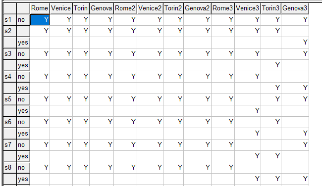
This has a little bit more info than we need: we only need the "yes" rows. This "yes"-only part is stored in set ps. It looks like:

Set ps
It looks like we are missing solution s1 here. That is because GAMS stores everything sparse. A row without any Y elements is just not stored. The bottom of set ps looks like:

Bottom of set ps
Indeed we have all 4096 solutions (well, except for that funny first row).

1.2 Form our X parameters


With this we can form our \(x_{s,i}\in \{0,1\}\) parameter. We want a 0-1 parameter for two reasons: we want numerical values to evaluate our objectives, and we need this parameter later on to use a filter tool.

*
* make a parameter out of this
*
parameter x(s,i) 'solutions';
x(s,i) = ps(s,i);
* make sure row 1 exists: introduce an EPS
x(s,i)$(
ord(s)=1 and ord(i)=1) = eps;
display x;


A trick to make the row not disappear is to insert an EPS value. An EPS value is like a zero when operated upon. But it exists: GAMS will no longer assume the whole row does not exist. 

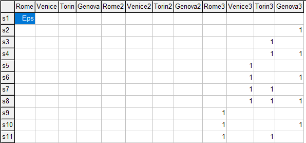
Parameter x with EPS value

1.3 Form the F values


Now we have all possible solutions in the \(x\) space, we can start calculating the \(f\) values: the objectives. 

table data(i,k) '### data set with 12 items'
            
cost   hours  people
   
Rome     1000    5       5
   
Venice    200    1      10
   
Torin     500    3       2
   
Genova    700    7       8
   
Rome2    1020    5       6
   
Venice2   220    1      10
   
Torin2    520    3       2
   
Genova2   720    7       4
   
Rome3    1050    5       5
   
Venice3   250    1       8
   
Torin3    550    3       8
   
Genova3   750    7       8
;
data(i,
'items') = 1;

parameter f(s,k) 'objective values';
f(s,k) =
sum(i, data(i,k)*x(s,i));
display f;


First we need to introduce our data. One objective is missing from the columns: the items. This is simply a column with ones: each item counts as one. With this we can calculate all \(f\) values in one swoop. The display output looks like:


----     56 PARAMETER f  objective values

             cost       hours      people       items

s1            EPS         EPS         EPS         EPS
s2        750.000       7.000       8.000       1.000
s3        550.000       3.000       8.000       1.000
s4       1300.000      10.000      16.000       2.000
s5        250.000       1.000       8.000       1.000
s6       1000.000       8.000      16.000       2.000
s7        800.000       4.000      16.000       2.000
s8       1550.000      11.000      24.000       3.000
s9       1050.000       5.000       5.000       1.000
s10      1800.000      12.000      13.000       2.000

. . . 

s4089    5930.000      37.000      52.000       9.000
s4090    6680.000      44.000      60.000      10.000
s4091    6480.000      40.000      60.000      10.000
s4092    7230.000      47.000      68.000      11.000
s4093    6180.000      38.000      60.000      10.000
s4094    6930.000      45.000      68.000      11.000
s4095    6730.000      41.000      68.000      11.000
s4096    7480.000      48.000      76.000      12.000

I only show the head and the tail of the display here. As we can see, some objective values violate the constraints. E.g. the last solution s4096, needs 76 people while we only have 50 available.

1.4 Constraint handling


We need to remove all solutions that violate the constraints. This can be done as follows:

parameter UpperLimit(k) 'bounds'/
  
cost 10000
  
hours  100
  
people  50
/;
upperlimit(k)$(upperlimit(k)=0) =
INF;

set infeas(s) 'infeasible solutions';
infeas(s) =
sum(k$(f(s,k)>UpperLimit(k)),1);

scalar numfeas 'number of feasible solutions';
numfeas =
card(s)-card(infeas);
display numfeas;

* kill solutions that are not feasible
x(infeas,i) = 0;
f(infeas,k) = 0;


This code removes all infeasible solutions from \(x\) and \(f\). Note that assigning a zero makes the corresponding records disappear: this is because GAMS stores everything sparse. The display shows:


----     71 PARAMETER numfeas              =     3473.000  number of feasible solutions


1.5 Filter out dominated solutions


In the result set there are quite a few dominated solutions. A solution \(f_1\) dominates \(f_2\) if:

  1. All objectives are better or equal
  2. There is one objective which is strictly better
Looking again at some of our solutions


----     87 PARAMETER f  objective values

             cost       hours      people       items

s1            EPS         EPS         EPS         EPS
s2        750.000       7.000       8.000       1.000
s3        550.000       3.000       8.000       1.000
s4       1300.000      10.000      16.000       2.000
s5        250.000       1.000       8.000       1.000
s6       1000.000       8.000      16.000       2.000
s7        800.000       4.000      16.000       2.000

we see that for this small subset

  • s1 is non dominated 
  • s5 dominates s2 and s3
  • s7 dominates s4 and s6
Remember we are minimizing cost, hours and people while maximizing items. 


GAMS has a tool to filter large data sets, call mcfilter.

D:\projects>mcfilter
No input file specified

Usage: mcfilter xxx.gdx

mcfilter will remove duplicate and dominated points in a
multi-criteria solution set.

The input is a gdx file with the following data:
   parameter X(point, i):   Points containing binary values.
                            If all zero for a point, use EPS.
   parameter F(point, obj): Objectives for the points X.
                            If all zero for a point, use EPS.
   parameter S(obj):        Direction of each objective: 1=max,-1=min
The output will be a gdx file called xxx_res.gdx with the same parameters
but without duplicates and dominated points.

D:\projects>


The X and the F parameters conform to our parameters. So the only thing to add are the signs of the objectives.

parameter sign(k) 'sign: -1:min, +1:max' /
  
(cost,hours,people) -1
  
items               +1
/;

execute_unload "feassols",x,f,sign=s;
execute "mcfilter feassols.gdx";


We see:


mcfilter v3.
Number of records     =     3473
Number of X variables =       12
Number of F variables =        4
Loading GDX data      =       15 ms
After X Filter, count =     3473
X Duplicate filter    =        0 ms
After F Filter, count =       83
F Dominance filter    =        0 ms
Writing GDX data      =        0 ms

There are 83 non-dominated or Pareto optimal solutions.

The final Pareto set looks like:

Non-dominated solutions

I list here the \(x\) values and the \(f\) values. As can be expected, a solution with all \(x_i=0\) is part of the Pareto set: doing nothing is very cheap; no other solution can beat this on price. Interestingly, project Genova3 is never selected.

Approach 2: use a series of MIP models


There is another way to generate these 83 points: use a MIP model. Or rather a series of MIP models. We use an algorithm like:

  1. Generate an optimal MIP solution. If infeasible: STOP.
  2. Add constraints: new solutions must be better in one objective
  3. Go to step 1.
This approach will be shown in part 2.


Conclusion


We have described a small multi-objective problem. We established that:
  • There are 4096 total combinations possible.
  • After removing the infeasible solutions, there are 3473 solutions left.
  • After removing the dominated solution, we are left with 83 Pareto optimal solutions. 
We used some less well-known GAMS tools in our script: a power set generator and a multi-criteria filter.

References


Monday, April 1, 2019

Math Checker?

Spell checkers are very useful. It may not be such a bad idea to have something like a "Math checker". It could flag things like:


References

  1. Bashiri, M. & Karimi, H. J, Effective heuristics and meta-heuristics for the quadratic assignment problem with tuned parameters and analytical comparisons, J Ind Eng Int (2012) 8: 6. https://doi.org/10.1186/2251-712X-8-6