R: plotly and R Markdown

In (1) I showed how we can produce a dynamic Gantt chart in R using the plotly package. What about if we put this in an R markdown document? If we knit the document to HTML there is no problem. We see something like:

Now the question arises what happens when I produce a PDF (through LaTeX)? Interestingly that works: we get a static picture:

Obviously we cannot run JavaScript based interaction in a PDF file. Same thing with Word output:

References

1. Gantt chart with R/plotly, http://yetanothermathprogrammingconsultant.blogspot.com/2017/03/gantt-chart-with-rplotly.html

Cutting Stock Problem: Generating all patterns by MIP Solution Pool

In (1) a small cutting stock problem is described. We need to cut up raw material rolls of width 5600 mm into the following pieces:

In this post I want to explore how we can use the solution pool technology in Cplex and Gurobi to do some of the heavy lifting for us.

Generating all possible patterns

From (1):

There are 308 possible patterns for this small instance.

Enumerating those patterns can be done by writing your own algorithm in your favorite programming language. Alternatively we can develop a small MIP model and let the solution pool do the job for us. See (2) for another example of this.

A minimalistic model is:

\[\bbox[lightcyan,10px,border:3px solid darkblue]{\begin{align}\min\>&0\\                              &L \le \sum_j w_j y_j \le R\\                              &y_j \in \{0,1,2,\dots,q_j\}\end{align}}\]

were \(w_j,q_j\) are the width and rolls from the demand table above, \(R=5600\), and \(L=\displaystyle\min_j w_j\).

There is a dummy objective: we are just looking for feasible solutions. The lower limit of \(L\) is there to exclude a pattern with all \(y_j=0\).

The solution pool will be able to find all feasible integer solutions for this model very fast.

When we solve this with GAMS/Cplex we see:

Total (root+branch&cut) =    0.13 sec. (4.46 ticks) Dumping 308 solutions from the solution pool...

This model is probably shorter than anything we can program in a standard programming language. 

Now we have a collection of all patterns \(a_{i,j}\) formed by collecting all \(y_j\) we found. Note that we enumerated literally all possible patterns including things like:

E.g. pattern 1 has only one item: a single roll with a width of 1380 mm.

Solving the cutting stock problem: minimize waste

The subsequent cutting stock problem can be formulated as (1):

\[\bbox[lightcyan,10px,border:3px solid darkblue]{\begin{align}\min\>&\sum_i c_i x_i\\                             &\sum_i a_{i,j} x_i \ge q_j\>\>\forall j\\                             &x_i \in \{0,1,2,\dots\}\end{align}} \]

The cost coefficients \(c_i\) correspond to cost or waste of each pattern \(i\), i.e. \(c_i = R-\displaystyle\sum_j w_j a_{i,j}\). 

Actually this model is not completely correct. Some of the patterns have a zero waste, E.g.:

These two patterns have a total width of \(1520+1880+2200=1520+1930+2150=5600\). As a result the model can use any amount of these patterns without cost. Indeed I saw a strange solution:

----    109 VARIABLE x.L  p18     14,    p38     10,    p40      4,   p68  99999,    p70     16,    p81  99999,    p142     4,    p159     8 p187     2

Indeed these two "zero waste" patterns have bad values.

We can correct this easily by changing the model to:

\[\bbox[lightcyan,10px,border:3px solid darkblue]{\begin{align}\min\>&\mathit{waste} = \sum_i c_i x_i\\                             &\sum_i a_{i,j} x_i = q_j\>\>\forall j\\                             &x_i \in \{0,1,2,\dots\}\end{align}} \]

i.e. use an equality constraint. Now we get a proper solution:

----    109 VARIABLE x.L  p18   6,    p30   1,    p38   8,    p40   7,    p68   5,    p70  15,    p75   1,    p81   4,    p121  4,    p142  7 p156  5,    p228  6,    p277  1,    p282  3 ----    114 PARAMETER n                    =           73  total amount of stock used ----    118 PARAMETER waste_percent        =        0.401  waste as percentage of material

Here we calculated:

\[\begin{align}&n=\sum_i x^*_i\\                     &\mathit{waste}\% = 100 \frac{\mathit{waste}^*}{n\cdot R}\end{align}\]

The numbers for total used raw material and percentage waste are the same as mentioned in (1).

Multiple solutions

The optimal combination of patterns to cut is not unique. One interesting subset of solutions is the one with a minimum number of different patterns. One way to find this solution is by solving a subsequent model, with the optimal amount of raw as constraint:

\[\bbox[lightcyan,10px,border:3px solid darkblue]{\begin{align}\min\>&\mathit{numPatterns} = \sum_i \delta_i\\                             &\sum_i a_{i,j} x_i = q_j\\                             &\sum_i x_i = n\\                             &x_i \le n \delta_i\\                             &\delta_i \in \{0,1\}\\                             &x_i \in \{0,1,2,\dots\}\end{align}}\]

This gives indeed what we want: 10 different patterns:

----    139 VARIABLE numPatterns.L         =           10  ----    139 VARIABLE x.L  p40   7,    p43   3,    p68   8,    p70  11,    p81   6,    p115 10,    p123  2,    p142 12,    p228 12,    p280  2

What about generating all possible optimal solutions for this? In (1) it is stated there are 19 solutions with 10 different patterns. Again we can use the solution pool for this. We see:

Total (root+branch&cut) =    3.22 sec. (794.99 ticks) Dumping 19 solutions from the solution pool...

Minimize number of raw material rolls

Instead of minimizing waste we can also just minimize the number of raw material rolls. This corresponds to \(c_i=1\). Solving the cutting stock model with this objective gives the same result.

In this case we can actually make the model much smaller by only considering “full” patterns. That is, only consider patterns that have no extra space left for another item from our demand data set.

From our original example:

we only want to keep rows that are non-dominated (the pattern numbers are reordered, so they don’t correspond):

The model to generate these can be written as:

\[\bbox[lightcyan,10px,border:3px solid darkblue]{\begin{align}\min\>&0\\                              &r = R-\sum_j w_j y_j\\                              &y_j \ge (1-\delta_j)  q_j&\forall j\\                              &r \le w_j \delta_j + R(1- \delta_j)&\forall j\\                              &r \ge 0\\                              &\delta_j \in \{0,1\}\\                              &y_j \in \{0,1,2,\dots,q_j\}\end{align}}\]

The binary variable \(\delta_j\in\{0,1\}\) is forced to assume the value of one when we still have a demand left for another item \(j\). We require that the remaining space available is smaller than the space needed to place any remaining demand.

Note that the second constraint \(y_j \ge (1-\delta_j)  q_j\) implements the implication:

\[y_j<q_j  \Rightarrow \delta_j=1\]

while the third constraint \(r \le w_j \delta_j + R(1- \delta_j)\) yields:

\[0 \le r \le \min_{j|\delta_j=1}w_j\]

and so forcing the remaining space \(r\) to be smaller than any demanded item we still can assign. When we solve this model with the solution pool we find just 213 different patterns (compared to 308 before). The subsequent cutting stock model can look like:

\[\bbox[lightcyan,10px,border:3px solid darkblue]{\begin{align}\min\>&n=\sum_i x_i\\                             &\sum_i a_{i,j} x_i \ge q_j\>\>\forall j\\                             &x_i \in \{0,1,2,\dots\}\end{align}} \]

We find the same \(n=73\) as before:

----    199 PARAMETER n                    =           73  total amount of stock used ----    199 VARIABLE x.L  p21  16,    p26   6,    p48   3,    p94   8,    p102  3,    p106 12,    p117  2,    p124  7,    p131  1,    p135  1 p188 12,    p208  2,    p228  1,    p280  2

Conclusion

The solution pool technique can be a useful tool for smaller instances of cutting stock problems where we want to enumerate patterns or optimal solutions. Of course for large problems these enumeration steps are not practical.

References

1. Cutting stock problem, https://en.wikipedia.org/wiki/Cutting_stock_problem
2. Employee Scheduling III: generating all shifts using the Cplex solution pool, http://yetanothermathprogrammingconsultant.blogspot.com/2017/01/employee-scheduling-iii-generating-all.html 

Joins in GAMS, SQL or R

To produce the charts in (1) I needed to do a multiple join on some data. From the GAMS model in (2) we extract the the following data:

sets   j 'tasks'  /job1*job10/   t 'stages' /t1*t10/ ; parameters    proctime(j,t) 'processing times for each stage'    machine(j,t) 'machine numbers for each stage (zero based)' ; variable x(j,t) 'start time of subtask';

What we want to arrive in R is the following:

i.e. a single data frame with slightly renamed columns (and a new column called end indicating when a sub-job finishes).

I used “approach 1” (pure SQL, described next) in (1), but there are other ways to attack the problem. I’ll describe a few.

Approach 1: pure SQL

Writing this into a SQLite database is very simple:

execute_unload "ft10"; execute "gdx2sqlite -i ft10.gdx -o ft10.db";

The database will contain a copy of all the data in the model, including the symbols we are interested in.

When loading the data we need to do two things:

1. Join proctime, machine and x on (j,t)
2. GAMS only stores non-zero elements, which we need to “repair”
3. Add the end column.

The second issue can be illustrated by looking at the table machine:

We miss the records that have a zero value. We can reintroduce them as follows. First we can generate the Carthesian product of J × T using a simple SQL subquery:

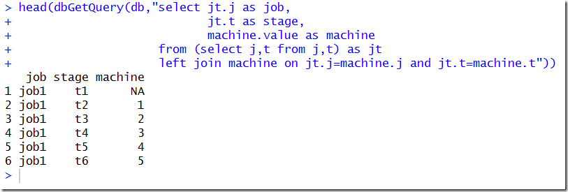
Note that table j has a single column j and table t has a single column t. As we have 10 jobs and 10 stages, this Carthesian product yields a table of 100 rows. Adding the machine number to this table is easy with a left join where we join on (j,t):

The left join added the machine column but the missing values are represented by NA in R (or NULL in SQL). This is easily fixed:

We now add the other columns and also calculate the end column:

Approach 2: GAMS + SQL

It is easy in GAMS to do the join. In addition we can use a trick to keep the zeroes:

alias(*,job,stage,attribute); parameter report(job,stage,attribute); report(j,t,'machine') = EPS + machine(j,t); report(j,t,'start') = EPS + x.l(j,t); report(j,t,'duration') = EPS + proctime(j,t); report(j,t,'end') = EPS + x.l(j,t) + proctime(j,t); execute_unload "ft10"; execute "gdx2sqlite -i ft10.gdx -o ft10.db";

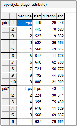
The EPS is a placeholder for the zero values The GAMS parameter report looks like:

The GDX2SQLITE tool will map the EPS values into zero before storing them in the database, so on the R side we see:

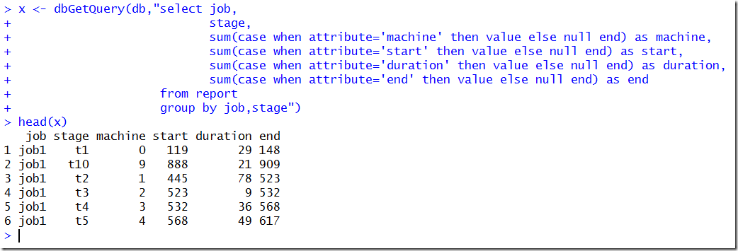
We need to pivot on the attribute, value columns. Unfortunately this is not completely trivial in SQL. A standard way to do this is:

Approach 3: GAMS + R

We keep the GAMS part the same:

alias(*,job,stage,attribute); parameter report(job,stage,attribute); report(j,t,'machine') = EPS + machine(j,t); report(j,t,'start') = EPS + x.l(j,t); report(j,t,'duration') = EPS + proctime(j,t); report(j,t,'end') = EPS + x.l(j,t) + proctime(j,t); execute_unload "ft10"; execute "gdx2sqlite -i ft10.gdx -o ft10.db";

On the R side we can read the parameter report as is and pivot using spread from the tidyr package:

Arguably this is the cleanest solution.

References

1. Gantt Chart with R/Plotly, http://yetanothermathprogrammingconsultant.blogspot.com/2017/03/gantt-chart-with-rplotly.html
2. Playing with job shop problem ft10 (1), http://yetanothermathprogrammingconsultant.blogspot.com/2014/04/playing-with-ft10-job-shop-1.html
3. Pivoting a table: GAMS, SQLite, R and Python, http://yetanothermathprogrammingconsultant.blogspot.com/2016/01/pivoting-table-gams-sqlite-r-and-python.html

Gantt Chart with R/Plotly

Plotly (1) is a great graphics library for producing dynamic plots. It also has an R interface. A simple example of a Gantt chart with R/plotly is shown in (2). Here is a more complicated version: a job shop problem with 10 jobs and 10 stages (3).

 

The colors correspond to the machine used in each stage. Machines are numbered 0…9.

 

References

1. Plotly: https://plot.ly/
2. https://www.r-bloggers.com/gantt-charts-in-r-using-plotly/
3. Playing with job shop problem ft10 (1), http://yetanothermathprogrammingconsultant.blogspot.com/2014/04/playing-with-ft10-job-shop-1.html

Binomial

In a nonlinear model I needed to use the following expression in a model equation:

\[y = \binom{x}{k}p^k(1-p)^{(x-k)}\]

Here \(x\) is the only decision variable. The integer version of “n choose k” is well known:

\[\binom{n}{k} = \frac{n!}{k!(n-k)!}\]

For fractional values we can generalize this to:

\[\binom{x}{y} = \frac{\Gamma(x+1)}{\Gamma(y+1)\Gamma(x-y+1)}\]

where \(\Gamma(.)\) indicates the gamma function, defined by

\[\Gamma(z) = \int_0^{\infty}x^{z-1}e^{-x} dx\]

In GAMS we have the binomial(x,y) function for this. The problem is that \(x\) can become rather large, while \(k\) is a small integer, say \(k=0,\dots,4\). For some values of \(x\) this leads to very inaccurate results and even overflows in subsequent calculations.

E.g.: 

scalars   x /112.8/   k /2/ ; parameter y; y("binomial") = binomial(x,k); y("log") = exp(loggamma(x+1)-loggamma(k+1)-loggamma(x-k+1)); display y;

yields the wrong result:

----      8 PARAMETER y  binomial 1.0000E+299,    log         6305.520

The logarithmic version is correct.

Instead of using the logarithmic version:

\[\binom{x}{k} = \exp\left(\log\Gamma(x+1)-\log\Gamma(k+1)-\log\Gamma(x-k+1)\right)\]

we can also exploit that \(k\) is a small integer. From:

\[\Gamma(z+1)=z\Gamma(z)\]

we have:

\[\begin{align}\binom{x}{k}&=\frac{x(x-1)\cdots(x-k+1)\Gamma(x-k+1)}{k!\Gamma(x-k+1)}\\ &=\frac{x(x-1)\cdots(x-k+1)}{k!}\\ &=\frac{\displaystyle\prod_{i=1}^k (x-i+1)}{k!}\end{align}\]

In GAMS:

scalars   x /112.8/   k /2/ ; parameter y; y("binomial") = binomial(x,k); y("log") = exp(loggamma(x+1)-loggamma(k+1)-loggamma(x-k+1)); set i /1*2/; y("prod") = prod(i,x-i.val+1)/fact(k); display y;

with results:

----     10 PARAMETER y  binomial 1.0000E+299,    log         6305.520,    prod        6305.520

I used this last “product” version in the model.

Note that the overflow in the binomial function does not happen for all (or even most) large values:

scalars   x /1112.8/   k /2/ ; parameter y; y("binomial") = binomial(x,k); y("log") = exp(loggamma(x+1)-loggamma(k+1)-loggamma(x-k+1)); set i /1*2/; y("prod") = prod(i,x-i.val+1)/fact(k); display y;

gives:

----     10 PARAMETER y  binomial 618605.520,    log      618605.520,    prod     618605.520

Dynamic Documents and their importance

When a model is ran say every few months and a report has to be produced based on the model results, a copy-paste like modus operandi can easily cause synchronization errors: the wrong text is inserted not referring to the current results but to an older simulation result. I recently had a discussion with someone from a government agency who experienced exactly this problem.

A similar thing can and does happen when documenting a piece of software: examples, code fragments or screen dumps refer to older versions of the program.

R and Rstudio provide tools to create dynamic documents from R using a nice Rstudio environment. We could have said in the document something like:

A cost savings of `r round(100*(oldcost-cost)/oldcost,1)`% has been achieved.

which would generate:

       A cost savings of 25.4% has been achieved.

Here we evaluated an R expression using data from the R session associated with the R markdown document.

Literate Programming

This is the grand-daddy of R Markdown. LP (Literate Programming) was meant to document source code, or rather have a single design document that could spit out either TeX for typesetting the document or Pascal (and later C) source code (4,5). Actually in some respects this tool was very flexible: things could be documented out-of-order. The name web was used for this. Knuth emphasized the usefulness of this: the order of thinking and writing about code is different than the order of generated source code. R Markdown prefers code chunks to be in order.

R users will appreciate the assignment symbol in LP:

 

R Markdown

The markup language to write documents in R is simple and somewhat restricted (6). Actually that may be a good thing. Too many ways to change the lay out of a document often leads to a somewhat less clean, more convoluted final product. Writing documentation while writing code is a big step forward I think. It makes it more pleasant to use and also has a beneficial impact on the code quality (explaining what you try to do helps to focus the mind and gets things better organized). I have heard people advancing the argument that documentation should be written before the code is written, but that looks to me not always a feasible or easy approach.

Recently better support for large documents (e.g. books) has been added in the form of being able to work sub-documents (sections or chapters) individually. Some books produced this way are shown at https://bookdown.org/.

Output formats

The main output formats of R Markdown are HTML, LaTeX, and MS Word. MS Word is especially important in non-academic institutions as Word and more general Office is a main work horse there. Click on the figures to enlarge.

 

Here is HTML, LaTeX and Word output of the same small example document.

Tables

Outputting tables is somewhat of a challenge. The easiest is to use the function kable. The LaTex and Word output is reasonable, but the HTML output needs some adjustment:

Books

References

1. Yihui Xie, Dynamic Documents with R and knitr, 2nd ediition, Chapmand and Hall/CRC, 2015.
2. Yihui Xie, bookdown, Authoring Books and Technical Documents with R Markdown, Chapman and Hall/CRC, 2016. Also available through: https://bookdown.org/yihui/bookdown/
3. Christopher Gandrud, Reproducible Research with R and RStudio, Chapman and Hall/CRC, 2015
4. Donald Knuth, Literate Programming, http://www.literateprogramming.com/knuthweb.pdf, paper on LP (LP means Literate Programming in this context and not Linear Programming).
5. Donald Knuth, Literate Programming, CSLI publications, 1992 (the book)
6. https://www.rstudio.com/wp-content/uploads/2015/02/rmarkdown-cheatsheet.pdf a short document summarizing R Markdown.

Employee Scheduling IV: direct optimization

In (1) a small employee scheduling problem is proposed. It is solved by first generating all possible shifts for each employee, and then solving a very simple MIP (Mixed Integer Programming) model to select the optimal combination of employees and shifts.

The optimization model is organized around a binary variable \(x_s \in \{0,1\}\) defined by:

\[x_s = \begin{cases}1 & \text{if shift $s$ is selected}\\                               0 & \text{otherwise} \end{cases}\]

and is very straightforward:

\[\begin{align}\min\>&\sum_s c_s x_s\\                           &\sum_{s|E(e,s)} x_s \le 1\>\forall e\\                           &\sum_{s|S(s,t)} x_s \ge R_t \> \forall t\\                             &x_s \in\{0,1\}\end{align}\]

Here \(E(e,s)\) indicates if shift \(s\) is done by employee \(e\), \(S(s,t)\) indicates if time period \(t\) is covered by shift \(s\) and \(R_t\) is the required staffing during period \(t\). The first constraint makes sure every employee is doing at most one shift in the 24-hour planning period. The second constraint establishes that we have enough staffing in each (hourly) period. Of course we try to minimize total cost.

In (2) we replicated the model in GAMS, using GAMS code to generate all possible shifts. In (4) we used a different technique to generate all shifts: the Cplex solution pool. In (3) we don’t generate all shifts in advance, but use a delayed column generation scheme to generate attractive shifts on the fly.

Here I try to show that we can attack the problem also in a very different way: directly optimize the selection of employees to use and the hours they work. A basic model to generate a single feasible shift for this problem is shown in (4) and (3). In those (sub-)models a binary variable \(w_t \in \{0,1\}\)  is used to indicate if an employee is working at period \(t\). For our “direct” model we extend this to:

\[w_{e,t} = \begin{cases}1 & \text{if employee $e$ works during period $t$}\\                               0 & \text{otherwise} \end{cases}\]

Again we first calculate the set canwork(e,t) indicating the time slots employee e can work. Furthermore we have parameters minlen(e) and maxlen(e) that tell us the minimum and maximum length of a shift for a given employee. Also the problem states that a shift is contiguous, i.e. no holes in the shift.

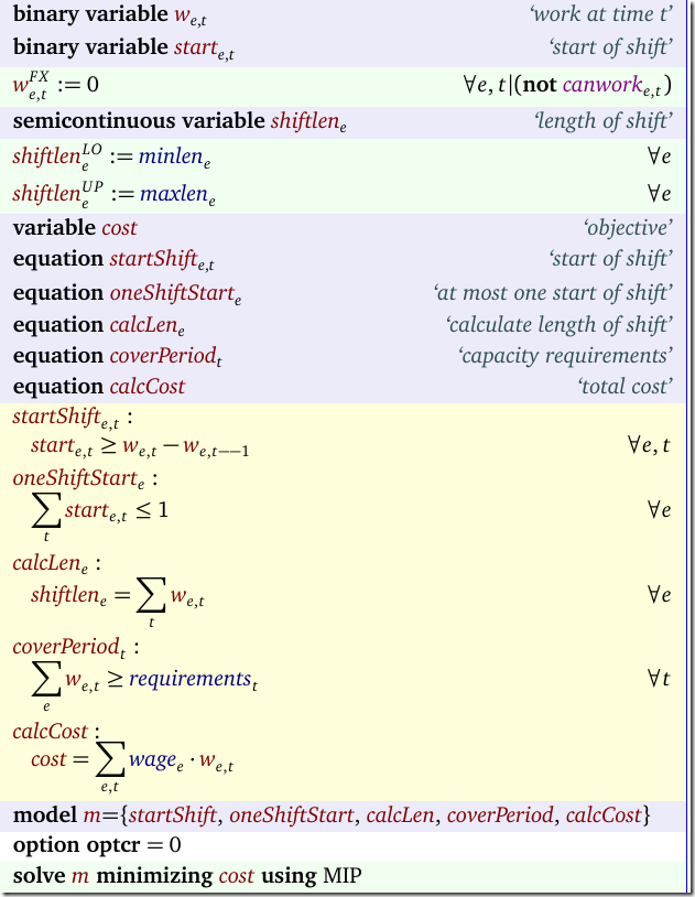
A MIP model can look like:

Notes:

• We fix \(w_{e,t}=0\) when canwork(e,t) is not true.
• The variable shiftlen(e) is a semi-continuous variable. It can be zero, or between minlen(e) and maxlen(e).
• If you don’t want to use semi-continuous variables, we can use binary variables \(\delta_e\) instead, and apply the constraint:
  

  \[\begin{align}&minlen_e \cdot \delta_e \le shiftlen_e \le maxlen_e \cdot\delta_e\\ &\delta_e \in \{0,1\}\\& shiftlen \ge 0\end{align}\]

  where shiftlen is now a positive variable. In GAMS we need to split this into two inequalities.
• The binary variable start(e,t) indicates when a shift starts. We observe this when w(e,t) switches from zero to one. A standard formulation is \(start_{e,t} \ge w_{e,t} – w_{e,t-1}\). As we need to wrap around hour 24: hour 1 minus 1 is hour 24, we use the GAMS \(—\) operator: \(start_{e,t} \ge w_{e,t} – w_{e,t--1}\).
• We only allow up to one start to enforce that we have no breaks in a shift: shifts are contiguous in this model.

We rely on the presolver of the MIP solver to remove all fixed variables from the model. I am old-fashioned and I prefer to not even generate the variables that are not needed. This requires a little bit of attention. The new model can look like:

binary variables    w(e,t) 'work at time t'    start(e,t) 'start of shift' ; semicont variables    shiftlen(e)  'length of shift' ; shiftlen.lo(e) = minlen(e); shiftlen.up(e) = maxlen(e); variable cost 'objective'; equations    startShift(e,t)     'start of shift'    oneShiftStart(e)    'at most one start of shift'    calcLen(e)          'calculate length of shift'    coverPeriod(t)      'capacity requirements'    calcCost            'total cost' ; startShift(canwork(e,t))..    start(e,t) =g= w(e,t) - w(e,t--1)$canwork(e,t--1); oneShiftStart(e)..    sum(canwork(e,t),start(e,t)) =l= 1; calcLen(e)..    shiftLen(e) =e= sum(canwork(e,t), w(e,t)); coverPeriod(t)..    sum(canwork(e,t), w(e,t)) =g= requirements(t); calcCost..    cost =e= sum(canwork(e,t), wage(e)*w(e,t)); model m /all/; option optcr=0; solve m minimizing cost using mip;

In this model I “protected” the use of \(w_{e,t}\) by canwork(e,t) in all cases. Note that in equation startShift the expression

w(e,t--1)$canwork(e,t--1) evaluates to zero when \(w_{e,t—1}\) does not correspond to canwork(e,t--1) being true. That is exactly what we want: if canwork(e,t) if false, implicitly we want the corresponding \(w_{e,t}=0\). We can verify the correct behavior by inspecting the equation listing in GAMS:

---- startShift  =G=  start of shift startShift(SMITH,t7)..  - w(SMITH,t7) + start(SMITH,t7) =G= 0 ; (LHS = 0)      startShift(SMITH,t8)..  w(SMITH,t7) - w(SMITH,t8) + start(SMITH,t8) =G= 0 ; (LHS = 0)      startShift(SMITH,t9)..  w(SMITH,t8) - w(SMITH,t9) + start(SMITH,t9) =G= 0 ; (LHS = 0)      REMAINING 415 ENTRIES SKIPPED

The first version of the model has the following statistics:

MODEL STATISTICS BLOCKS OF EQUATIONS           5     SINGLE EQUATIONS          545 BLOCKS OF VARIABLES           4     SINGLE VARIABLES          981 NON ZERO ELEMENTS         3,381     DISCRETE VARIABLES        918

while the second version shows:

MODEL STATISTICS BLOCKS OF EQUATIONS           5     SINGLE EQUATIONS          483 BLOCKS OF VARIABLES           4     SINGLE VARIABLES          857 NON ZERO ELEMENTS         2,942     DISCRETE VARIABLES        856

Results

This model solves quickly (it is small), and we find an optimal solution with a cost of 4670. The schedule looks like:

 

We see one shift wrapping at t24: Employee Davis. The optimal solution is not unique. In (1) and (2) different solutions are obtained (with the same total cost). The optimal solution has no slack in staffing: we exactly match the staffing requirements:

References

1. Loren Shure, Generating an Optimal Employee Work Schedule Using Integer Linear Programming, January 6, 2016, http://blogs.mathworks.com/loren/2016/01/06/generating-an-optimal-employee-work-schedule-using-integer-linear-programming/ describes the problem with a Matlab implementation.
2. Employee Scheduling I: Matlab vs GAMS, http://yetanothermathprogrammingconsultant.blogspot.com/2017/01/employee-scheduling-i-matlab-vs-gams.html has a GAMS version of the model in (1).
3. Employee Scheduling II : Column Generation, http://yetanothermathprogrammingconsultant.blogspot.com/2017/01/employee-scheduling-ii-column-generation.html uses a Column Generation approach to solve this problem.
4. Employee Scheduling III: generating all shifts using the Cplex solution pool, http://yetanothermathprogrammingconsultant.blogspot.com/2017/01/employee-scheduling-iii-generating-all.html uses the Cplex Solution Pool technology to generate all possible shifts. This is an alternative approach to the method shown in this post.