In an earlier post I read a GAMS variable into Python program. Here I add some more notes on the tools and procedures we can use for this.
In this example we want to convert a long table coming from a GAMS model, into a wide dataframe for further processing in R or Python.
This operation is not very unusual. With the right tools, it is not so difficult to perform this task.
1. GAMS: Export to GDX and dump into SQLite
We are interested in variable loc which is declared as:
positive variable loc(k,c) 'location of sensor';
After the solve we do a display of loc.L (i.e. the levels) and we see:
---- 36 VARIABLE loc.L location of sensor
x y
k1 0.893 0.893
k2 0.668 0.318
k3 0.137 0.786
k4 0.139 0.316
The data is displayed here as a matrix. We can also display it in a list format, which resembles more how the data will be stored in a GDX file or a typical “long” database table:
---- 39 VARIABLE loc.L location of sensor
k1.x 0.893
k1.y 0.893
k2.x 0.668
k2.y 0.318
k3.x 0.137
k3.y 0.786
k4.x 0.139
k4.y 0.316
Here we just use two different display styles to show the same data. Later on we will see that data can also be actually stored in these two formats. This applies to database tables and R or Python dataframes.
To store the loc variable in an SQLite database we can use the following in the GAMS model:
As we will see below, the variable does not only store the level but also the lower and upperbound and the marginal.execute_unload 'results.gdx';
execute 'gdx2sqlite -i results.gdx -o results.db -fast';
2. SQLite in R: RSQLite
In R we can use the RSQLite package to read data from SQLite databases:
> library(RSQLite)Loading required package: DBI> sqlite<-dbDriver("SQLite")
> db <- dbConnect(sqlite,"c:\\projects\\tmp\\code\\results.db")
> dbListTables(db)[1] "c" "cov" "covk"
[4] "i" "iscovered" "iscoveredk"
[7] "j" "k" "loc"
[10] "p" "radius" "scalarequations"
[13] "scalars" "scalarvariables"
> dbGetQuery(db,"select * from loc")
k c level lo up marginal
1 k1 x 0.8934478 0 1 1.942971e-12
2 k1 y 0.8934479 0 1 1.942972e-12
3 k2 x 0.6683234 0 1 -3.541285e-13
4 k2 y 0.3176426 0 1 -7.418214e-13
5 k3 x 0.1372328 0 1 -1.447327e-12
6 k3 y 0.7863548 0 1 -3.002015e-13
7 k4 x 0.1388778 0 1 -1.699826e-12
8 k4 y 0.3156270 0 1 -7.479254e-13
Note that the table and resulting dataframe are in “long” format. To select the x and y coordinates we need to do something like:
In the following sections we will try to get x and y as columns in one single dataframe.> x <- dbGetQuery(db,"select k,level as x+ from loc+ where c='x'")> y <- dbGetQuery(db,"select k,level as y+ from loc+ where c='y'")> xk x1 k1 0.89344782 k2 0.66832343 k3 0.13723284 k4 0.1388778> yk y1 k1 0.89344792 k2 0.31764263 k3 0.78635484 k4 0.3156270
3. Pivot in SQL
A big advantage of SQL is that we can do some data manipulation steps before creating and populating the dataframe. In this case we want to do a pivot operation where the level column becomes two columns x and y. Of course we can do that in SQL. There are many ways to implement this, and here is an example:
> dbGetQuery(db,"select tx.k as k, tx.level as x, ty.level as y+ from (select k,level from loc where c='x') as tx,+ (select k,level from loc where c='y') as ty+ where tx.k=ty.k")k x y1 k1 0.8934478 0.89344792 k2 0.6683234 0.31764263 k3 0.1372328 0.78635484 k4 0.1388778 0.3156270
A simpler and faster SQL query is:
> dbGetQuery(db,"
+   select k,
+          sum(case when c='x' then level else null end) as x,
+          sum(case when c='y' then level else null end) as y
+   from loc
+   group by k")
   k         x         y
1 k1 0.8934478 0.8934479
2 k2 0.6683234 0.3176426
3 k3 0.1372328 0.7863548
4 k4 0.1388778 0.3156270
Note: There is an SQL PIVOT construct. As of now it seems supported only by SQL Server and Oracle.
4. Pivot in R: reshape2
The pivot operation can also be performed in R. Here we use the dcast function of the reshape2 package:
> library(reshape2)> df1<-dbGetQuery(db,"select k,c,level from loc")> df1k c level1 k1 x 0.89344782 k1 y 0.89344793 k2 x 0.66832344 k2 y 0.31764265 k3 x 0.13723286 k3 y 0.78635487 k4 x 0.13887788 k4 y 0.3156270> df2<-dcast(df1,k~c,value.var="level")> df2k x y1 k1 0.8934478 0.89344792 k2 0.6683234 0.31764263 k3 0.1372328 0.78635484 k4 0.1388778 0.3156270
5. Pivot in R: tidyr
The tidyr package is a successor to reshape2. The function we use to pivot our data is called spread:
> library(tidyr)> df1<-dbGetQuery(db,"select k,c,level from loc")> df1k c level1 k1 x 0.89344782 k1 y 0.89344793 k2 x 0.66832344 k2 y 0.31764265 k3 x 0.13723286 k3 y 0.78635487 k4 x 0.13887788 k4 y 0.3156270> spread(df1,c,level)k x y1 k1 0.8934478 0.89344792 k2 0.6683234 0.31764263 k3 0.1372328 0.78635484 k4 0.1388778 0.3156270
6. SQLite in Python
In Python we use packages SQLite3 and of course pandas.
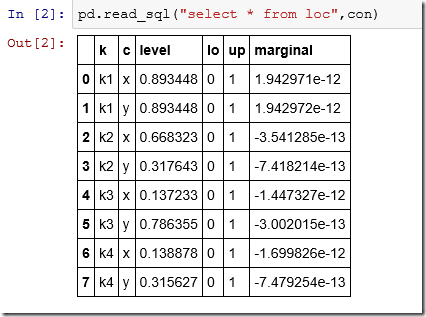
There is no built-in “list tables” function so we use the master table of the SQLite database. The table loc looks like:
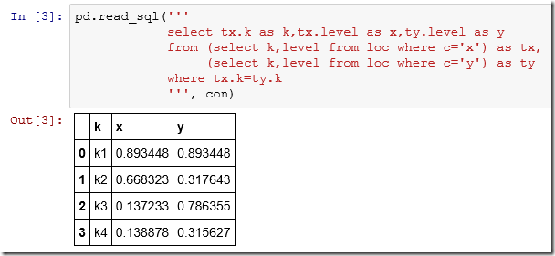
The SQL “pivot” query is long so we can use a multi-line string:
7. Pivot in Python: pandas.pivot
Pandas has a sophisticated pivot method:
The output is not exactly the same as with the SQL approach, but it is close. We just need to do one more step to make the index labels k a normal data column:
Conclusion
When we move data from GAMS –> SQLite –> dataframe, we often need to make some data manipulation steps, some of which may not be totally trivial. But we have powerful and flexible tools at our disposal: SQL and R/Python. In this case we showed that a pivot operation to transform a “long” table into a “wide” one can be done either at the SQL level when importing the data into R/Python or directly in R/Python.
Update
Some timings on a larger data set are here.


No comments:
Post a Comment