Tuesday, February 28, 2017

Comparing two GAMS models

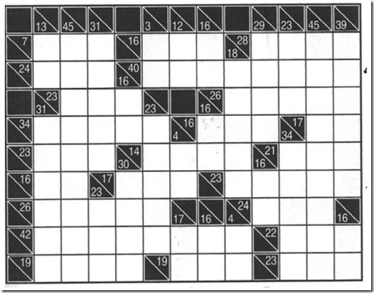
I see a lot of GAMS models. Some of them are really beautifully done. Others, I would like to suggest some edits. Here we compare two different models that solve a Kakuro puzzle. The problem from (1) is here:

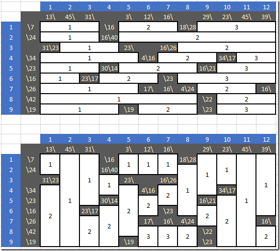
image

We need to fill in the white cells with numbers \(1,…,9\). Each horizontal or vertical region of consecutive white cells has to add up to the number in the black cell just above to to the left. Furthermore each number in each region has to be unique. The solution of the above puzzle is (again from (1)):

image

We have the following two models:

  • MODEL A: taken from (1). The appendix has a GAMS model.
  • MODEL B: developed independently by me, discussed in (2)

In the following I try to show things next to each other: MODEL A (1) at the left and MODEL B (2) to the right.

The differences between the models vary between mundane syntax or style issues, and more substantial differences in the underlying optimization model. In some cases I do things differently because of taste and customs, in others I may have a good reason to write things down differently.

MODEL A MODEL B
image

sets
  i
'rows'    /r1*r9/
  j
'columns' /c1*c12/
  k
'values'  /v1*v9/
  b
'blocks'  /block1*block47/

;

Instead of using numbers as set elements, I prefer to prefix them by a distinguishing (short) name. This is especially useful when displaying and viewing high-dimensional data. Of course we add some explanatory text. I prefer to put them in quotes to create a visual barrier between the set name and the explanatory text and because things like a comma can unexpectedly end an explanatory text without quotes. Many GAMS models create spurious sets, parameters etc. because there is a comma in the explanatory text.

The blocks or segments have a different numbering scheme. In model A we number them as follows:

image

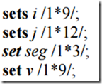
The maximum number of segments in a row or column is three, which explains the set seg in model A.

In model B the numbering scheme is global:

image

Here we have 47 different blocks. Somehow model A calls regions “segments” and in model B they are called “blocks”. 

MODEL A MODEL B
image  

I tend to keep variables together and put them after data entry and data manipulation. You will see the variable declarations in model B further down.

image  

The data structures in model A indicate the number of segments in each row (and column), their starting and end-position and the required summation value. This gives rise to eight different parameters.

image
image

* data entry
parameter block(b,i,j) /
* rows
   
block1.r1.(c1*c3)     7
   
block2.r1.(c5*c7)    16
   
block3.r1.(c9*c12)   28
   
...
   
block21.r9.(c1*c4)   19
   
block22.r9.(c6*c8)   19
   
block23.r9.(c10*c12) 23

* columns
   
block24.(r1*r2).c1  13
   
block25.(r4*r9).c1  31
   
block26.(r1*r9).c2  45
   
...
   
block45.(r1*r9).c11 45
   
block46.(r1*r6).c12 39
   
block47.(r8*r9).c12 16
 
/

;


* derived data
sets
  ij(i,j)
'cells to fill'
  sblock(b,i,j)
'mapping between b <-> (i,j)'
;
parameter bval(b) 'value of block';

bval(b) =
smax
((i,j),block(b,i,j));
sblock(b,i,j) = block(b,i,j);
ij(i,j)=
sum
(sblock(b,i,j),1);


The left model A has a lot of individual assignment statements. That is not the most compact way to initialize data. GAMS has parameter initialization syntax for this. E.g. we could have written the initialization of n_segs_l as:

parameter n_segs_l(i) /
   (2,3,7,8)    2
   (1,4,5,6,9)  3
/;
  

The right model B has just one parameter block that has all the needed information. This approach has just one mapping between block number \(k\) and a bunch of cells with coordinates \((i,j)\) and also has the summation value. In the derived data we extract data in a form that is easier to use in the rest of the model.

image  

This looks like a somewhat unusual approach. I will discuss this further down at the spot where these equations are defined.

MODEL A MODEL B
image

binary variable x(i,j,k) 'assignment';
integer variable v(i,j) 'cell values'
;
v.lo(ij) = 1;
v.up(ij) = 9;

variable dummy 'dummy objective'
;

Remember that Model A had binary variable a_bin(i,j,v) declared earlier. Model B has an extra variable \(v\) which will help us keeping the equations simpler and also to reduce the number of non-zero elements in the LP matrix \(A\).

The naming of identifiers (names of sets, parameters, variables and equations) is somewhat a matter of taste. Admittedly, \(x\) is not the most self-descriptive name, but I like it if there is a single central variable that really plays a dominating role the model. Often I like to use a naming scheme where I use very short names for identifiers that are used a lot, and longer, more descriptive names for identifiers less often used in the model. That would imply, my equation names are longer:

equation declarations are not listed

equations
   oneval(i,j) 
'each white cell has one value'
   unique(b,k) 
'values are unique inside a block'
   defval(i,j) 
'calculate value of cell'
   sumblock(b) 
'summation of cells inside a block'
   edummy      
'dummy objective'

;

The equations are defined below:

image

oneval(ij(i,j))..
  
sum(k, x(i,j,k)) =e= 1;

Model A is putting this constraint on each black and white cell. Hence it is a \(\le\) constraint. This is somewhat of a disadvantage as the solution is no longer unique, and we need an objective to help us preventing zero values in the white cells. A better formulation is in model B where we run only over the white cells and thus can use a \(=\) constraint. This will yield a stronger MIP formulation.

image
image

unique(b,k)..
  
sum(sblock(b,i,j),x(i,j,k)) =l= 1;

Model A has a complex equation, because it tries to find all line segments in a row \(i\). In Model B we have a much simpler equation that is actually more powerful: it handles both the row and column blocks in one swoop. I like to make the equations as simple as possible as equations are more difficult to debug. The set sblock helps us to simplify this constraint. By definition sblock only refers to white cells.

MODEL A MODEL B
image defval(ij(i,j))..
   v(i,j) =e=
sum(k, ord
(k)*x(i,j,k));

sumblock(b)..
  
sum
(sblock(b,i,j), v(i,j)) =e= bval(b);

On the left we have again a very complicated equation for the row segments. On the right we split the logic in two parts: the first equation calculates the integer value \(v_{i,j}\) of a cell \((i,j)\). The second equation sums up the values in a block \(b\) and make sure this sum has the correct value. This equation handles both row-wise blocks and column-wise blocks. Note again that we only operate on the white cells.

Each white cell \((i,j)\) is part of two blocks (row and column). By introducing an intermediate variable \(v_{i,j}\) I prevent duplication of the expression \(\sum_k k\cdot x_{i,j,k}\). This formulation makes the model larger but sparser.
image  

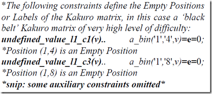
Here the model A introduces a lot of equations to force the “black” cells to zero.

First, this is not my preferred way to do this. We can make a subset black(i,j) (containing the coordinates of all black cells) and then just say:

undefined_value(black(i,j),v).. a_bin(i,j,v) =e= 0;

Of course we can do this more compactly by setting bounds instead of using a full-blown equation:

a_bin.fx(black(i,j),v) = 0;

Even better is just not generate any variable with \((i,j)\) outside the white cells. In model B we have created a convenient set for that: \(IJ(i,j)\): this subset has only the “white” cells. I make sure all equations only operate on the white cells and never touch the black cells. This requires a little bit more thought and discipline but I prefer this approach.

image  

In model B we handled these constraints already as we dealt with row and column-wise blocks in one single constraint.

MODEL A MODEL B
image

edummy..
   dummy =e= 0;


model m /all/;
solve
m using mip minimizing dummy;

option
v:0;
display
v.l;

On the left we have a real objective to prevent zeroes in the white cells. Probably we should add

option optcr=0;

to force the MIP solver to find the global optimum with a gap of zero. Note that MODEL B does not need any optcr as we only look for a feasible integer solution.

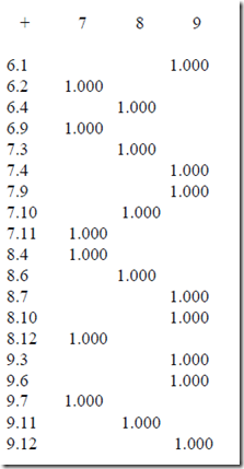
The display of a_bin.l is not very convenient to view. It looks like:

imageimage

imageimage

A better display can be achieved by:

parameter w(i,j);
w(i,j) =
sum(v,ord
(v)*a_bin.l(i,j,v));
option
w:0;
display
w;

That would lead to a similar output as produced by model on the right:

----    119 VARIABLE v.L  cell values

            c1          c2          c3          c4          c5          c6          c7          c8          c9

r1           4           2           1                       1           8           7                       8
r2           9           8           7                       2           4           9           1           7
r3                       6           8           9                                               5           9
r4           6           4           9           7           8                       9           2           5
r5           8           9           6                       2           1           7           4
r6           9           7                       8           6           3                       6           7
r7           5           1           8           9           3                                               9
r8           2           5           6           7           4           8           9           1
r9           1           3           9           6                       9           7           3

+         c10         c11         c12

r1           9           4           7
r2           8           3           6
r3           6           2           4
r4                       9           8
r5           7           5           9
r6           4           1           5
r7           8           7
r8           9           6           7
r9           6           8           9

The final question is: how do these models perform? I ran the problem with the open source solver CBC (1 thread):

MODEL A MODEL B
Search completed - best objective -88, took 32349 iterations and 854 nodes (14.82 seconds) Search completed - best objective 0, took 215 iterations and 0 nodes (0.68 seconds)

As expected a MIP solver prefers the tighter formulation of MODEL B.

Notes
  • Model B is much more compact. We can quantify this as follows: Model A has about 432 lines, Model B 119 lines. This includes data entry.
  • Model A uses the ord(.) function 12 times, Model B only uses the ord(.) function once. Often models with lots of ord()’s are more likely to be messy models.
References
  1. José Barahona da Fonseca, A novel linear MILP model to solve Kakuro puzzles, 2012. http://www.apca.pt/publicacoes/6/paper56.pdf (This is referred to as MODEL A)
  2. MODEL B is: http://yetanothermathprogrammingconsultant.blogspot.com/2017/02/solving-kakuro-puzzles-as-mip.html
Friday, February 24, 2017

Python Optimization Modeling: optlang

Example with Transportation Model from (1) taken from the optlang docs:

from optlang import Variable, Constraint, Objective, Model

# Define problem parameters
# Note this can be done using any of Python's data types. Here we have chosen dictionaries
supply = {"Seattle": 350, "San_Diego": 600}
demand = {"New_York": 325, "Chicago": 300, "Topeka": 275}

distances = {  # Distances between locations in thousands of miles
    "Seattle": {"New_York": 2.5, "Chicago": 1.7, "Topeka": 1.8},
    "San_Diego": {"New_York": 2.5, "Chicago": 1.8, "Topeka": 1.4}
}

freight_cost = 9  # Cost per case per thousand miles

# Define variables
variables = {}
for origin in supply:
    variables[origin] = {}
    for destination in demand:
        # Construct a variable with a name, bounds and type
        var = Variable(name="{}_to_{}".format(origin, destination), lb=0, type="integer")
        variables[origin][destination] = var

# Define constraints
constraints = []
for origin in supply:
    const = Constraint(
        sum(variables[origin].values()),
        ub=supply[origin],
        name="{}_supply".format(origin)
    )
    constraints.append(const)
for destination in demand:
    const = Constraint(
        sum(row[destination] for row in variables.values()),
        lb=demand[destination],
        name="{}_demand".format(destination)
    )
    constraints.append(const)

# Define the objective
obj = Objective(
    sum(freight_cost * distances[ori][dest] * variables[ori][dest] for ori in supply for dest in demand),
    direction="min"
)
# We can print the objective and constraints
print(obj)
print("")
for const in constraints:
    print(const)

print("")

# Put everything together in a Model
model = Model()
model.add(constraints)  # Variables are added implicitly
model.objective = obj

# Optimize and print the solution
status = model.optimize()
print("Status:", status)
print("Objective value:", model.objective.value)
print("")
for var in model.variables:
    print(var.name, ":", var.primal)

Some other Python based options are Pulp, Pyomo and PyMathprog (2).

References
  1. G.B.Dantzig, Linear Programming and Extensions, Princeton University Press, 1963
  2. PyMathProg: another Python based modeling tool: http://yetanothermathprogrammingconsultant.blogspot.com/2016/12/pymathprog-another-python-based.html 

Tuesday, February 21, 2017

Multiplication of binary with continuous variable between zero and one

A small tidbit.

The standard linearization for the multiplication of two binary variables \(z=x \cdot y\) with \(x,y \in \{0,1\}\) is:

\[\boxed{\begin{align}&z\le x\\&z \le y\\& z\ge x+y-1\\&z \in \{0,1\}\end{align}}\]

What about if \(y\) is continuous between zero and one, \(y\in[0,1]\) (while \(x\) remains a binary variable)? In that case we can use the formulation in (1) where we consider a continuous variable \(y \in [y^{lo},y^{up}]\):

\[\boxed{\begin{align}&\min\{0,y^{lo}\} \le z \le \max\{0,y^{up}\} \\
&y^{lo} \cdot x \le z \le y^{up} \cdot x \\
&y − y^{up} \cdot (1 − x) \le z \le y − y^{lo} \cdot (1 − x)\end{align}}\]

When we plug in \(y^{lo}=0\) and \(y^{up}=1\), we end up with the same thing:

\[\boxed{\begin{align}&z\le x\\&z \le y\\& z\ge x+y-1\\&z \in [0,1]\end{align}}\]

We can easily verify the correctness by checking what happens when \(x=0\) or \(x=1\):

\[\begin{align}
    &x=0 & \implies & \begin{cases}
                              z\le 0\\
                              z \le y &\text{(NB)}\\
                              z \ge y-1 &\text{(NB)} \\
                              z \in [0,1]
                             \end{cases} & \implies  & z=0 \\
    &x=1 & \implies & \begin{cases}
                              z\le 1 & \text{(NB)}\\
                              z \le y \\
                              z \ge y \\
                              z \in [0,1]
                             \end{cases} & \implies  & z=y
\end{align}\]

where \(\text{NB}\) means non-binding by which I mean we can ignore this constraint.

References
  1. Multiplication of a continuous and a binary variable, http://yetanothermathprogrammingconsultant.blogspot.com/2008/05/multiplication-of-continuous-and-binary.html

Saturday, February 18, 2017

Solving Kakuro puzzles as a MIP

The Kakuro puzzle is another logical puzzle similar to Sudoku, KenKen and Takuzu. A small example from (1) is:

image 

The rules are as follows:

  1. Each (white) cell must be filled with a value \(1,..,9\).
  2. Each (white) cell belongs to a horizontal and/or a vertical block of contiguous cells.
  3. The values of the cells in each block add up to a given constant. These constants are to the left (or top) of the block. A notation a\b is used: a is the sum for the block below and b is the sum for the block to the right.
  4. The values in each block must be unique (i.e. no duplicates).
Model

The actual model is rather simple. Similar to (2) and (3) I define a binary decision variable:

\[x_{i,j,k} = \begin{cases}1 & \text{if cell $(i,j)$ has the value $k$} \\
     0& \text{otherwise}\end{cases}\]

where \(k=\{1,..,9\}\). Of course, we can select only one value in a cell, i.e.:

\[ \sum_k x_{i,j,k} = 1 \>\>\forall i,j|IJ(i,j)\]

where \(IJ(i,j)\) is the set of white cells we need to fill in. To make the model simpler we also define an integer variable \(v_{i,j}\) with the actual value:

\[v_{i,j} = \sum_k k\cdot x_{i,j,k}\]

The values in each block need to add up the given constant. So:

\[\sum_{i,j|B(b,i,j)} v_{i,j} = C_b \>\>\forall b\]

where the set \(B(b,i,j)\) is the mapping between block number and cells \((i,j)\). The uniqueness constraint is not very difficult at all:

\[\sum_{i,j|B(b,i,j)} x_{i,j,k} \le 1 \>\>\forall b,k\]

Note that (1) uses a different numbering scheme for the cells, but otherwise the models are very similar. My version of the model is smaller in terms of nonzero elements in the matrix, due to my use of intermediate variables \(v_{i,j}\).

Data entry

A compact way to enter the data for the example problem in GAMS is:

parameter
  block(b,i,j)
/
   
block1.r1.(c1*c2)   16  ,   block13.(r1*r3).c1  23
   
block2.r1.(c5*c7)   24  ,   block14.(r6*r7).c1  11
   
block3.r2.(c1*c2)   17  ,   block15.(r1*r4).c2  30
   
block4.r2.(c4*c7)   29  ,   block16.(r6*r7).c2  10
   
block5.r3.(c1*c5)   35  ,   block17.(r3*r7).c3  15
   
block6.r4.(c2*c3)    7  ,   block18.(r2*r3).c4  17
   
block7.r4.(c5*c6)    8  ,   block19.(r5*r6).c4   7
   
block8.r5.(c3*c7)   16  ,   block20.(r1*r5).c5  27
   
block9.r6.(c1*c4)   21  ,   block21.(r1*r2).c6  12
   
block10.r6.(c6*c7)   5  ,   block22.(r4*r7).c6  12
   
block11.r7.(c1*c3)   6  ,   block23.(r1*r2).c7  16
   
block12.r7.(c6*c7)   3  ,   block24.(r5*r7).c7   7
 
/

The sets \(IJ(i,j)\) and parameter \(C_b\) can be easily extracted from this.

Results

After adding a dummy objective, we can solve the model as a MIP (Mixed Integer Programming) Model. The output looks like:

----     75 VARIABLE v.L 

            c1          c2          c3          c4          c5          c6          c7

r1           9           7                                   8           7           9
r2           8           9                       8           9           5           7
r3           6           8           5           9           7
r4                       6           1                       2           6
r5                                   4           6           1           3           2
r6           8           9           3           1                       1           4
r7           3           1           2                                   2           1

It is noted that although I used the declaration \(x_{i,j}\), only the subset of cells that we actually need to fill in is used in the equations. GAMS will only actually generate the variables that appear in the equations, so all the “black” cells are not part of the model.

Cplex can solve the model in zero iterations and zero nodes: it solves the model completely in the presolve.

Interestingly in (1) somewhat disappointing performance results are reported. They use CBC and a solver called eplex (never heard of that one). I checked the above small instance with CBC and it can solve it in zero nodes, just like Cplex.

A large, difficult example

This example is taken from (4):

image

For this problem Cplex has to do a little bit of work. The log looks like:

---   3,665 rows  4,921 columns  19,189 non-zeroes
---   4,920 discrete-columns

. . .

Dual simplex solved model.

Root relaxation solution time = 0.44 sec. (102.53 ticks)

        Nodes                                         Cuts/
   Node  Left     Objective  IInf  Best Integer    Best Bound    ItCnt     Gap

      0     0        0.0000   325                      0.0000     1727        
      0     0        0.0000   188                    Cuts: 39     2562        
      0     0        0.0000   233                    Cuts: 49     3018        
      0     0        0.0000   227                    Cuts: 18     3403        
      0     0        0.0000   147                    Cuts: 64     4037        
*     0+    0                            0.0000        0.0000             0.00%
Found incumbent of value 0.000000 after 4.42 sec. (1071.33 ticks)
      0     0        cutoff              0.0000        0.0000     4423    0.00%
Elapsed time = 4.44 sec. (1072.36 ticks, tree = 0.01 MB, solutions = 1)

. . .

Proven optimal solution.

MIP Solution:            0.000000    (4423 iterations, 0 nodes)

To be complete, CBC takes a little more time:

Search completed - best objective 0, took 55117 iterations and 140 nodes (42.00 seconds)
Strong branching done 1748 times (104829 iterations), fathomed 9 nodes and fixed 122 variables
Maximum depth 18, 0 variables fixed on reduced cost

This model does not solve completely in the presolve. However the computation times look quite good to me, especially when compared to what is reported in (1).

The solution looks like:

image

Proving uniqueness

We can prove the uniqueness of this solution by adding the constraint:

\[\sum_{i,j,k|IJ(i,j)} x^*_{i,j,k} x_{i,j,k} \le |IJ| –1 \]

where \(x^*\) is the previously found optimal solution, and \(|IJ|\) is the cardinality of the set \(IJ(i,j)\) (i.e. the number of “white” cells). Note that \(\sum x^*_{i,j,k}=\sum x_{i,j,k} = |IJ|\). With this constraint we should either find a different solution (so the solution was not unique), or the model should be declared “infeasible”.

References
  1. Helmut Simonis, Kakuro as a Constraint Problem, Cork Constraint Computation Centre (4C), University College Cork, 2008.
  2. MIP Modeling: From Sukodu to Kenken via Logarithms, http://yetanothermathprogrammingconsultant.blogspot.com/2016/10/mip-modeling-from-sudoku-to-kenken.html 
  3. Solving Takuzu puzzles as a MIP using xor, http://yetanothermathprogrammingconsultant.blogspot.com/2017/01/solving-takuzu-puzzles-as-mip-using-xor.html
  4. http://pagesperso.g-scop.grenoble-inp.fr/~cambazah/page1/page7/assets/data_generated_hard.ecl has some larger data sets.
  5. http://www.gecode.org/doc-latest/MPG.pdf, Chapter 21 is about solving Kakuro using Gecode, a constraint programming solver.
  6. José Barahona da Fonseca, A novel linear MILP model to solve Kakuro puzzles, 2012. This has a (partial) GAMS model (stylistically I would write things differently; the model can be written more cleanly).