Monday, January 29, 2018

Linearizing nested absolute values

In [1] an interesting question is posted: How to model a nested absolute value: \[ \min \left| \left( |x_1-a_1| \right) - \left( |x_2-a_2|\right) \right| \] A standard way to model absolute values in the objective function in a linear minimization model \[\min |x|\] is: \[\begin{align}\min\>&y\\&-y \le x \le y\end{align}\] It would be tempting to apply this here: \[\begin{align}\min\>&z\\&-z\le y_1-y_2 \le z\\& -y_i \le x_i - a_i \le y_i \end{align}\] The easiest way to illustrate this formulation is wrong, is showing a counter example. For this I added a few extra conditions to the model:\[\begin{align}\min\>&z\\&-z\le y_1-y_2 \le z\\& -y_i \le x_i - a_i \le y_i\\&x_1=x_2\\&x_1,x_2 \in [2,5] \end{align}\] When using \(a_1 = -1\), \(a_2=2\), I see as solution:

----     37 PARAMETER a  

i1 -1.000,    i2  2.000


----     37 VARIABLE x.L  

i1 2.000,    i2 2.000


----     37 VARIABLE y.L  

i1 3.000,    i2 3.000


----     37 VARIABLE z.L                   =        0.000  

We can see the value  \(y_2=3\) is incorrect: \(|x_2-a_2|=|2-2|=0\). The underlying reason is of course: we are not minimizing the second term \(|y_2-a_2|\).

A correct formulation will need extra binary variables (or something related such as a SOS1 construct):\[\begin{align}\min\>&z\\&-z\le y_1-y_2 \le z\\& y_i \ge x_i - a_i \\& y_i \ge -(x_i - a_i)\\ & y_i \le x_i - a_i + M\delta_i\\& y_i \le -(x_i - a_i) + M(1-\delta_i)\\&\delta_i \in \{0,1\}  \end{align}\]

Background


The function \(z = \max(x,y) \) can be linearized as: \[\begin{align}&z \ge x\\&z \ge y\\ &z \le x + M\delta\\&z \le y + M(1-\delta)\\&\delta \in \{0,1\}\end{align}\] The function \(z=|x|\) can be interpreted as \(z=\max(x,-x)\).

Results


The example model now will show:


----     68 VARIABLE x.L  

i1 2.000,    i2 2.000


----     68 VARIABLE y.L  

i1 3.000


----     68 VARIABLE z.L                   =        3.000  

----     68 VARIABLE d.L  

                      ( ALL       0.000 )


I think we need binary variables for for both terms \(y_i\) although for this numerical example it seems that we could only do it for the second term \(y_2\), and handle \(y_1\) as before, I believe that is just luck. A correct formulation will use binary variables for both inner absolute values.

Linearizing absolute values is not always that easy.

References


Tuesday, January 23, 2018

Knuth and SAT

Presentation by Knuth about SAT problems and solvers (and also a little bit about Integer Programming). Not new but still interesting..


Section 7.2.2.2 is about SAT. Ran out of extra space for more sub-numbering:


Looks like Donald Knuth got a bit sidetracked by this subject (his program SAT13 seems to indicate he implemented at least 13 SAT solvers). He had the same thing when starting on the book TAOCP. He did not like any of the available typesetting software. So he implemented TeX. Then he did not like the fonts, so he implemented MetaFont. There is a similar story about about Bill Orchard-Hays: he needed to implement an LP solver on a different machine. In those times everything was coded in assembly. Well, he did not like the assembler, so he started with implementing a proper macro-assembler. Then he did not like the linker, so he implemented a new linker. After that it just took a few weeks to implement the LP solver. (I am not sure this story is 100% true, but it could well be).

Knuth mentions integer programming and Cplex when discussing pictures like:


References


  1. Donald E. Knuth, The Art of Computer Programming, Volume 4, Fascicle 6, Satisfiability, 2015
  2. William Orchard-Hays, Advanced Linear Programming Computing Techniques, 1968.

Thursday, January 18, 2018

CBC and semi-continuous variables

The Coin CBC MIP solver [5] does not seem to have a way to specify semi-continuous variables in either an LP file or an MPS file [1] (slightly edited):

Hi,

I am using version 2.9.9 of cbc in ubuntu 17.10 docker image.  My test.lp file has following content:

Maximize
 obj: x1 + 2 x2 + 3 x3 + x4
Subject To
 c1: - x1 + x2 + x3 + 10 x4 <= 20
 c2: x1 - 3 x2 + x3 <= 30
 c3: x2 - 3.5 x4 = 0
Bounds
  0 <= x1 <= 40
  2 <= x4 <= 3
General
 x4
Semis
 x1 x2 x3

When trying with semis section I get an error "terminate called after throwing an instance of 'CoinError?' Aborted"

On a Mac I get: libc++abi.dylib: terminating with uncaught exception of type CoinError? Abort trap: 6 

However if I comment out Semis it works fine. I was hoping that Semis are supported. Am I doing something wrong?

My command is : cbc -presolve on -import test.lp solve solu out.txt

On further analysis I found out when in cbc prompt I type "import test.lp" it fails and shows same error is I tried in MPS format as well there i got

Bad image at line 19 < SC BND1 YTWO 3 >

Contents of mps file are :

NAME          TESTPROB
ROWS
 N  COST
 L  LIM1
 G  LIM2
 E  MYEQN
COLUMNS
    XONE      COST                 1   LIM1                 1
    XONE      LIM2                 1
    YTWO      COST                 4   LIM1                 1
    YTWO      MYEQN               -1
    ZTHREE    COST                 9   LIM2                 1
    ZTHREE    MYEQN                1
RHS
    RHS1      LIM1                 5   LIM2                10
    RHS1      MYEQN                7
BOUNDS
 UP BND1      XONE                 4
 SC BND1      YTWO                 3
ENDATA

Some notes:

  • The LP file parser crashes hard. Preferably, a parser should never crash on erroneous input and always produce a (good) error message,
  • The MPS file reader does not crash, but the error message "bad image" seems a bit strange to me (what has this to do with an image? In prehistoric times an "image" was sometimes used as the equivalent of "file". "Bad file" is still somewhat of a bad message.).
  • CBC actually supports semi-continuous variables.
  • Semi-continuous behavior can be modeled with binary variables [3]: \[\begin{align} &\delta \cdot \ell \le x \le \delta \cdot u\\&\delta \in \{0,1\}\\&x \in [0,u]\\&\ell > 0\end{align}\]
  • If you have good upper bounds, this may actually solve faster (MIP solvers do like binary variables).
  • Semi-continuous variables with a zero lower bound do not make much sense.
  • The LP and MPS file in this post do not represent the same problem.
  • Why did nobody complain about this before?
The answer by John Forrest [2] is funny:

Semi continuous variables are in Cbc (as a simple version of lotsizing variables).

However there is no way of inputting them using mps or lp files.

Having invented semi-continuous variables (probably before you were born!), I feel some responsibility to make them easier to use in Cbc. I will get them working with mps files in trunk.

 John Forrest


References

Monday, January 15, 2018

Least squares as QP: convexity issues

This is a post about theory vs practice. Theory says: least squares problems are convex. In practice we can encounter cases where this is not the case. The background is a post [1] about a non-negative least squares problem being solved using Cplex's matlab interface (function cplexlsqnonneglin [2]). It fails. We will fix this by modeling: a somewhat non-intuitive reformulation will help us solving this problem.

Model 1


The model this function tries to solve is:
\[\begin{align}\min\>&||Cx-d||_2^2\\&x\ge 0\end{align}\]
Unfortunately we see:


Number of nonzeros in lower triangle of Q = 861
Using Approximate Minimum Degree ordering
Total time for automatic ordering = 0.00 sec. (0.02 ticks)
Summary statistics for factor of Q:
  Rows in Factor            = 42
  Integer space required    = 42
  Total non-zeros in factor = 903
  Total FP ops to factor    = 25585
CPLEX Error  5002: objective is not convex.
QP with an indefinite objective can be solved
to local optimality with optimality target 2,
or to global optimality with optimality target 3.
Presolve time = 0.03 sec. (0.06 ticks)
Barrier time = 0.03 sec. (0.06 ticks)

This looks like a numerical or tolerance issue: least-squares problems should be convex. More on this further down.

Model 2


I often propose a different model:
\[\begin{align}\min\>&||r||_2^2\\&r=Cx-d\\&x\ge 0, r\text{ free}\end{align}\]
This looks like a bad idea: we add variables \(r\) and extra constraints. However this model has a big advantage: the \(Q\) matrix is much more well-behaved. It is basically a (very well-scaled) diagonal matrix. Using this model we see:


Tried aggregator 1 time.
QP Presolve eliminated 1 rows and 1 columns.
Reduced QP has 401 rows, 443 columns, and 17201 nonzeros.
Reduced QP objective Q matrix has 401 nonzeros.
Presolve time = 0.02 sec. (1.21 ticks)
Parallel mode: using up to 8 threads for barrier.
Number of nonzeros in lower triangle of A*A' = 80200
Using Approximate Minimum Degree ordering
Total time for automatic ordering = 0.00 sec. (3.57 ticks)
Summary statistics for Cholesky factor:
  Threads                   = 8
  Rows in Factor            = 401
  Integer space required    = 401
  Total non-zeros in factor = 80601
  Total FP ops to factor    = 21574201
 Itn      Primal Obj        Dual Obj  Prim Inf Upper Inf  Dual Inf          
   0   3.3391791e-01  -3.3391791e-01  9.70e+03  0.00e+00  4.20e+04
   1   9.6533667e+02  -3.0509942e+03  1.21e-12  0.00e+00  1.71e-11
   2   6.4361775e+01  -3.6729243e+02  3.08e-13  0.00e+00  1.71e-11
   3   2.2399862e+01  -6.8231454e+01  1.14e-13  0.00e+00  3.75e-12
   4   6.8012056e+00  -2.0011575e+01  2.45e-13  0.00e+00  1.04e-12
   5   3.3548410e+00  -1.9547176e+00  1.18e-13  0.00e+00  3.55e-13
   6   1.9866256e+00   6.0981384e-01  5.55e-13  0.00e+00  1.86e-13
   7   1.4271894e+00   1.0119284e+00  2.82e-12  0.00e+00  1.15e-13
   8   1.1434804e+00   1.1081026e+00  6.93e-12  0.00e+00  1.09e-13
   9   1.1163905e+00   1.1149752e+00  5.89e-12  0.00e+00  1.14e-13
  10   1.1153877e+00   1.1153509e+00  2.52e-11  0.00e+00  9.71e-14
  11   1.1153611e+00   1.1153602e+00  2.10e-11  0.00e+00  8.69e-14
  12   1.1153604e+00   1.1153604e+00  1.10e-11  0.00e+00  8.96e-14
Barrier time = 0.17 sec. (38.31 ticks)

Total time on 8 threads = 0.17 sec. (38.31 ticks)
QP status(1): optimal
Cplex Time: 0.17sec (det. 38.31 ticks)

Optimal solution found.
Objective :           1.115360

This reformulation is not only useful for Cplex. Some other solvers show the same behavior: the first model is declared to be non-convex while the second model solves just fine. Some other solvers solve both models ok. These solvers add a very tiny value to the diagonal elements of the \(Q\) matrix to make it numerically positive semi-definite [3].


A little background in numerics


The \(Q\) matrix is formed by \(C^TC\). We can show that \(C^TC\) is always positive semi-definite. This follows from: \[x^T(C^TC)x=(Cx)^T(Cx)=y^Ty\ge 0\] However the inner product \(Q=C^TC\) can accumulate some small floating point errors, causing \(Q\) to be no longer positive semi-definite. When I calculate \(Q=C^TC\) and print its eigenvalues I see:


 [1]  6.651381e+03  4.436663e+02  3.117601e+02  2.344391e+02  1.377582e+02  4.842287e+01
 [7]  2.471843e+01  4.970353e+00  4.283370e+00  3.878515e+00  9.313360e-01  4.146773e-01
[13]  2.711321e-01  2.437365e-01  2.270969e-01  8.583981e-02  2.784610e-02  2.047456e-02
[19]  1.670033e-02  8.465492e-03  3.948085e-03  2.352994e-03  1.726044e-03  1.287873e-03
[25]  1.095779e-03  2.341448e-04  1.776231e-04  1.266256e-04  4.064795e-05  2.980187e-05
[31]  1.056841e-05  2.409130e-06  2.039620e-06  5.597181e-07  1.367130e-07  2.376693e-08
[37]  3.535393e-09  1.355988e-11  2.996032e-14 -1.468230e-13 -1.622616e-13 -2.217776e-13

The presence of negative eigenvalues indicate this calculated matrix \(Q\) is indeed not pos def. Another verification is to see if we can form a Cholesky factorization [4]. This will fail if the matrix is not positive definite:


This type of factorization on the \(Q\) matrix is typically used inside Quadratic Programming solvers. Finally, it is noted that it is also possible that \(Q\) is actually positive definite but both tests (eigenvalues and Cholesky decomposition) fail to see this due to floating point errors inside their computations. Of course, for all practical purposes that means the matrix is not numerically positive definite.

In Ordinary Least Squares (OLS) it is well known that solving the normal equations is not very numerically stable. I believe this is related (the same inner product is formed).


André-Louis Cholesky (1875-1918)

Performance


This reformulation can also help with performance. For an example see [5].

References


  1. https://stackoverflow.com/questions/48164626/linear-combination-of-curves-to-match-a-single-curve-with-integer-constraints
  2. Cplex, cplexlsqnonneglinhttps://www.ibm.com/support/knowledgecenter/SSSA5P_12.8.0/ilog.odms.cplex.help/refmatlabcplex/html/cplexlsqnonneglin-m.html
  3. Gurobi, PSDtolhttp://www.gurobi.com/documentation/7.5/refman/psdtol.html
  4. Cholesky decomposition, https://en.wikipedia.org/wiki/Cholesky_decomposition
  5. Constrained Least Squares solution times II, http://yetanothermathprogrammingconsultant.blogspot.com/2016/11/constrained-least-squares-solution.html

Saturday, January 13, 2018

Solving a facility location problem as an MIQCP

Facility location models [1] are one of the most studied areas in optimization. It is still interesting to build a model from scratch.

The question is [2]:

Given \(m\) customer locations, find the minimum number of warehouses \(n\) we need such that each customer is within \(\mathit{MaxDist}\) miles from a warehouse.

Model 1 : minimize number of warehouses


The idea I use here, is that we assign a customer to a warehouse and make sure the distance constraint is met. In the following let \(i\) be the customers, \(j\) be the (candidate) warehouses. We can define the binary variable:\[\mathit{assign}_{i,j} = \begin{cases}1 & \text{if customer $i$ is serviced by warehouse $j$}\\0 &\text{otherwise}\end{cases}\]

A high-level distance constraint is:

\[\begin{align} &\mathit{assign}_{i,j}=1 \Rightarrow \mathit{Distance}(i,j) \le \mathit{MaxDist}&&\forall i,j \\ &\sum_j \mathit{assign}_{i,j} =1 && \forall i\\&\mathit{assign}_{i,j} \in \{0,1\} \end{align}\]

The distance is the usual:

\[ \mathit{Distance}(i,j)  = \sqrt{ \left( \mathit{dloc}_{i,x} - \mathit{floc}_{j,x} \right)^2 + \left( \mathit{dloc}_{i,y} - \mathit{floc}_{j,y} \right)^2 }  \]

Here \(\mathit{dloc}, \mathit{floc}\) are the \((x,y)\) coordinates of the demand (customer) and facility (warehouse) locations. The \(\mathit{dloc}\) quantities are constants, opposed to \(\mathit{floc}\) which are decision variables: these are calculated by the solver.

This distance function is nonlinear. We can make it more suitable to be handled by quadratic solvers by reformulating the distance constraint as:

\[\left( \mathit{dloc}_{i,x} - \mathit{floc}_{j,x} \right)^2 + \left( \mathit{dloc}_{i,y} - \mathit{floc}_{j,y} \right)^2 \le \mathit{MaxDist}^2 + M (1-\mathit{assign}_{i,j})\]

where \(M\) is a large enough constant.

The next step is to introduce a binary variable: \[\mathit{isopen}_{j} = \begin{cases}1 & \text{if warehouse $j$ is open for business}\\0 &\text{otherwise}\end{cases}\] We need \(\mathit{isopen}_j=0 \Rightarrow \mathit{assign}_{i,j} =0\). This can be modeled as: \[\mathit{assign}_{i,j}\le \mathit{isopen}_j\] The objective is to minimize the number of open warehouses:\[\min n = \sum_j \mathit{isopen}_j\]

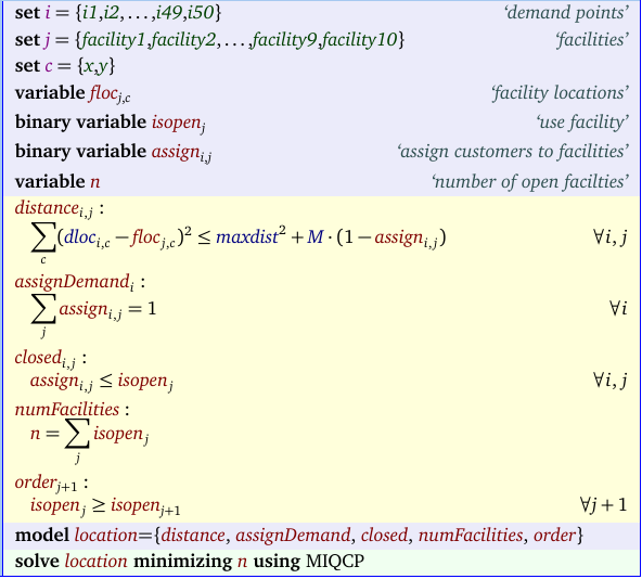
A complete model can look like:


The problem is a convex MIQCP: Mixed Integer Quadratically Constrained Problem. This model type is supported by solvers like Cplex and Gurobi. The last constraint order is designed to make sure the open facilities are the first in the list of candidate facilities. It is also a way to reduce symmetry in the model.

To test this, I generated 50 random points with \(x,y\) coordinates between 0 and 100. The maximum distance is \(\mathit{MaxDist}=40\). The optimal solution is:


----     60 VARIABLE n.L                   =        3.000  number of open facilties

----     60 VARIABLE isopen.L  use facility

facility1 1.000,    facility2 1.000,    facility3 1.000


----     63 PARAMETER locations  

                    x           y

facility1      43.722      25.495
facility2      31.305      59.002
facility3      67.786      51.790

It is noted that the only relevant result in the solution is \(n=3\) (the number of open facilities). The chosen location for the warehouses and the assignment is not of much value. We can see this from a picture of the solution, in particular the variables floc and assign:

Misinterpretation of the solution

Model 2: Optimal location of warehouses


We can solve a second model that given \(n=3\) warehouses obtains a solution that:

  • assigns customers to their closest warehouse
  • finds warehouse locations such that the distances are minimized 
If we minimize the sum of the distances:
\[\min \sum_{i,j} \left[ \mathit{assign}_{i,j}\cdot \sqrt{\sum_c  \left( \mathit{dloc}_{i,c} - \mathit{floc}_{j,c} \right)^2 }\right]\]
we achieve both goals in one swoop. Of course this is a nasty nonlinear function. We can make this a little bit more amenable to being solved with standard solvers:
\[\bbox[lightcyan,10px,border:3px solid darkblue]{\begin{align}\min &\sum_{i,j} d_{i,j}\\ &d_{i,j} \ge  \sum_c  \left( \mathit{dloc}_{i,c} - \mathit{floc}_{j,c} \right)^2 - M (1-\mathit{assign}_{i,j})&&\forall i,j\\&\sum_j \mathit{assign}_{i,j} =1 && \forall i\\&\mathit{assign}_{i,j} \in \{0,1\}\\&0\le d_{i,j}\le\mathit{MaxDist}^2 \end{align}}\] Note that now \(j = 1,\dots,n=3\). This is again a convex MIQCP model.

To be a little bit more precise: with this model we minimize the sum of the squared distances which is slightly different. The objective that models the true distances would look like \[\min\sum_{i,j} \sqrt{d_{i,j}}\] This would make the model no longer quadratic, so we would need to use a general purpose MINLP solver (or use some piecewise linear formulation). With the linear objective \(\min \sum_{i,j} d_{i,j}\) we place a somewhat higher weight on large distances. This is a different situation from the first model. There we also used the trick to minimize squared distances, but in that case it did not change the meaning of the model: it gives the same optimal solution. In the case of this second model the summation of squared distances will give slightly different results from actually minimizing the sum of distances.

When we solve this model we see a different location for the warehouses:


----     78 PARAMETER locations  

                    x           y

facility1      24.869      18.511
facility2      72.548      46.855
facility3      24.521      74.617

The plot looks much better now:

Optimal Warehouse Locations with Minimized Distances


There are of course many other ways to attack this problem:

  • Instead of using two models we can combine them. We can form a multi-objective formulation \(\min w_1 n  + w_2 \sum_{i,j} d_{i,j}\)  Use a large weight \(w_1\) to put priority on the first objective.
  • Instead of minimizing the sum of the distances we can choose to minimize the largest distance.
  • Instead of Euclidean distances we can use a Manhattan distance metric. This will give us a linear MIP model.


References 


  1. Zvi Drezner, Horst W. Hamacher, eds., Facility Location, Applications and Theory, Springer, 2001,
  2. Facility Location - Algorithm to Minimize facilities serving customers with distance constraint, https://stackoverflow.com/questions/48213881/facility-location-algorithm-to-minimize-facilities-serving-customers-with-dist

Friday, January 12, 2018

New book: linear programming using matlab


If you want to know more about the nitty-gritty details of linear programming solvers, this hefty book (637 pages) may be of interest. Contains lots of Matlab code that implement different LP solvers.

Contents


  1. Introduction
  2. Linear Programming Algorithms
  3. Linear Programming Benchmark and Random Problems
  4. Presolve Methods
  5. Scaling Techniques
  6. Pivoting Rules
  7. Basis Inverse and Update Methods
  8. Revised Primal Simplex Algorithm
  9. Revised Dual Simplex Algorithm
  10. Exterior Point Simplex Algorithm
  11. Interior Point Methods
  12. Sensitivity Analysis

    A. MATLAB's Optimization Toolbox Algorithms
    B. State-of-the-Art Linear Programming Solvers: CLP and Cplex 

References


Sunday, January 7, 2018

A difficult row selection problem

The problem


In [1] an interesting problem is posted. From a matrix \(A_{i,j}\) (\(i=1,\dots,m\),\(j=1,\dots,n\)) select \(K\) rows such that a cost function is minimized. Let \(S\) be the set of selected rows. The cost function is defined as: \[ \min_S \> \left\{ 0.2 \max_{i \in S} A_{i,1} + 0.4 \sum_{i \in S} A_{i,2} - 0.3 \sum_{i \in S} A_{i,3} - 0.1 \max_{i \in S} A_{i,4} \right\} \] This problem is by no means simple to model (probably unbeknownst to the poster). Let's dive in.

Selecting rows


We define a binary decision variable:
\[\delta_i = \begin{cases} 1 &\text{if row $i$ is selected}\\ 0 &\text{otherwise}\end{cases}\]
We want to select \(K\) rows:
\[\sum_i \delta_i = K \]

A simpler objective


If the cost function was just  \[ \min_S \> \left\{ 0.4 \sum_{i \in S} A_{i,2} - 0.3 \sum_{i \in S} A_{i,3} \right\} \] things are easy. We can write: \[\min\>  0.4 \sum_i \delta_i A_{i,2} - 0.3 \sum_i \delta_i A_{i,3}\]

As this cost function is separable in the rows, we can even use simple algorithm to solve problem (instead of using a MIP mode):
  1. Create a vector \(c_i =  0.4 A_{i,2} - 0.3 A_{i,3}\)
  2. Sort the vector \(c\) 
  3. Pick rows that correspond to the \(K\) smallest values of \(c\)
The \(\max\) terms in the objective make the objective non-separable in the rows, so this little algorithm is no longer applicable.

Review: Modeling a maximum


The maximum \(z = \max(x,y)\) where \(x\) and \(y\) are decision variables, can in general be modeled as: \[\bbox[lightcyan,10px,border:3px solid darkblue]{\begin{align} &z\ge x\\ &z \ge y\\ &z \le x + M \eta\\ & z\le y + M(1-\eta)\\ &\eta \in \{0,1\}\end{align}}\]

Here \(M\) is a large enough constant. This formulation can be interpreted as: \[\begin{align}&z \ge x \text{ and } z \ge y\\  &z \le x \text{ or } z \le y \end{align}\]

The maximum of a set of variables: \(z = \max_k x_k\) is a direct extension of the above: \[\bbox[lightcyan,10px,border:3px solid darkblue]{\begin{align} &z\ge x_k && \forall k\\  &z \le x_k + M \eta_k&& \forall k\\ & \sum_k \eta_k = 1\\ &\eta_k \in \{0,1\}\end{align}}\] This formulation is correct in all cases. We can simplify things a little bit depending on how the objective is written.

If we are minimizing the maximum we can actually simplify things considerably:\[\min \left\{\max_k x_k \right\} \Rightarrow \begin{cases}\min &z\\ &z \ge x_k & \forall k\end{cases}\]

Maximizing the maximum does not save much. We can write:
\[
\max \left\{  \max_k  x_k \right\}  \Rightarrow \begin{cases}\max   & z\\& z \le x_k+M \eta_k & \forall k\\ & \displaystyle \sum_k \eta_k = 1\\ &\eta_k \in \{0,1\}
\end{cases}\]

A complete model

We generate a small data set with 10 rows. We want to select \(K=2\) rows that maximize our objective. The data part of the model can look like:


The model itself using the most general implementation of the maximum can look like:


Notes:

  • The parameter range functions as a big-M constant.
  • The variables \(\eta_{i,j}\) are only used for the \(j\)'s corresponding to a "max" column.
  • We needed to make sure that the selected row with the maximum (i.e. \(\eta_{i,j}=1\)) is limited the selected rows. We do this by requiring \(\delta_j=0 \Rightarrow \eta_{i,j}=0\).
  • We can simplify things for the first objective where \(c_j>0\). For this column we have a simple "minimax" case. This means we can drop equations maxObj2, sum1, and implyZero and the corresponding \(\eta\)'s from the model. We still need them for the last column.
  • Similarly we can drop equation maxObj1 when  \(c_j < 0\) (objective 4).
  • An optimized model can therefore look like:


The results look like:


----     57 PARAMETER A  data

             j1          j2          j3          j4

i1       -6.565       6.865       1.008      -3.977
i2       -4.156      -5.519      -3.003       7.125
i3       -8.658       0.004       9.962       1.575
i4        9.823       5.245      -7.386       2.794
i5       -6.810      -4.998       3.379      -1.293
i6       -2.806      -2.971      -7.370      -6.998
i7        1.782       6.618      -5.384       3.315
i8        5.517      -3.927      -7.790       0.048
i9       -6.797       7.449      -4.698      -4.284
i10       1.879       4.454       2.565      -0.724


----     57 VARIABLE delta.L  select rows

i3 1.000,    i5 1.000


----     57 VARIABLE obj.L  single objectives

j1 -6.810,    j2 -4.994,    j3 13.341,    j4  1.575


----     57 VARIABLE z.L                   =       -7.519  final objective

The solution can also be viewed as:


The data set is small enough to enumerate all possible solutions. There are only 45 different ways to select two rows from ten, so we can just select the best objective:


As an aside, the different configurations were generated by letting the solution pool technology in Cplex enumerate all solutions to the optimization problem: \[ \begin{align} \min\>&0\\ & \sum_i x_i = K\\ & x_i \in \{0,1\} \end{align} \] This explains the somewhat strange ordering of the different solutions. Of course this overkill: if you have a hammer in the form of a solver, everything looks like an optimization problem.

A larger data set with \(m=10,000\) rows and \(K=100\) took 30 seconds to solve even though it has 20,000 binary variables. The number of combinations for this problem is \[{{m}\choose{K}} = \frac{m!}{(m-K)!K!} \] This is a big number for these values:

65208469245472575695415972927215718683781335425416743372210247172869206520770178988927510291340552990847853030615947098118282371982392705479271195296127415562705948429404753632271959046657595132854990606768967505457396473467998111950929802400

A little bit too big to try complete enumeration.

References


  1. https://stackoverflow.com/questions/48098198/choose-optimal-subset-of-size-k-given-certain-constraints-r

Wednesday, January 3, 2018

Variant of an Assignment Problem

The standard assignment problem can be stated as:

\[\bbox[lightcyan,10px,border:3px solid darkblue]{\begin{align}\min\>&\sum_{i,j} c_{i,j} x_{i,j}\\ & \sum_j x_{i,j} = 1 && \forall i\\ & \sum_i x_{i,j} = 1 && \forall j\\&x_{i,j} \in \{0,1\} \end{align}}\]

There are highly efficient specialized algorithms for this problem [1]. I often solve these problems just as an LP (the integer variables are automatically integer valued for this particular problem). That sounds like a dumb approach, but there are some reasons:

  • LP solvers are actually very good in solving this quickly (often faster than a specialized method that is not implemented with very much care for efficiency [2]).
  • Variants and extensions are (often) easily handled.

The standard model above assumes the sets \(i \in I\) (sources) and \(j \in J\) (destinations) have the same size. Let \(n=|I|\) and \(m=|J|\) be the number of \(i\)'s and \(j\)'s. Thus the standard model has \(n=m\). Now assume we have more \(j\)'s than \(i\)'s: \(m>n\). The model can be updated to:

\[\bbox[lightcyan,10px,border:3px solid darkblue]{\begin{align}\min\>&\sum_{i,j} c_{i,j} x_{i,j}\\ & \sum_j x_{i,j} = 1 && \forall i\\ & \sum_i x_{i,j} \le 1 && \forall j\\&x_{i,j} \in \{0,1\} \end{align}}\]

I.e. each \(i\) is connected to a unique \(j\), but some \(j\)'s are not assigned. A solution for a random data set with \(n=5\) and \(m=10\) can look like:


----     41 PARAMETER c  cost coefficients

            j1          j2          j3          j4          j5          j6          j7          j8          j9         j10

i1       0.661       0.756       0.627       0.284       0.086       0.103       0.641       0.545       0.032       0.792
i2       0.073       0.176       0.526       0.750       0.178       0.034       0.585       0.621       0.389       0.359
i3       0.243       0.246       0.131       0.933       0.380       0.783       0.300       0.125       0.749       0.069
i4       0.202       0.005       0.270       0.500       0.151       0.174       0.331       0.317       0.322       0.964
i5       0.994       0.370       0.373       0.772       0.397       0.913       0.120       0.735       0.055       0.576


----     41 VARIABLE x.L  assignment variables

            j2          j5          j6          j9         j10

i1                       1
i2                                   1
i3                                                           1
i4           1
i5                                               1

Let's add a picture to this post (created with tikz):
Original assignment and new variant


In [3] an unusual variant is asked for: the assigned \(j\)'s should be adjacent. The required configuration can be seen in the right picture above.

The first thing we do is to keep track if a \(j\) node is assigned. For this we introduce new binary variables \(y_j\) and replace the second assignment constraint \(\sum_i x_{i,j} \le 1\) by:

\[\begin{align} &y_j = \sum_i x_{i,j}\\&y_j \in \{0,1\}\end{align}\]

The variable \(y_j\) will be zero for the unassigned nodes (grey in the picture above), and one if connected (red). We can make sure we don't have "holes" in the \(y\) vector by requiring that we see the pattern \([0,\> 1]\)  only once. This we can model as:

\[\begin{align} &z_j \ge y_j - y_{j-1}\\& \sum_j z_j \le 1\\&z_j \in \{0,1\} \end{align}\]

This approach is often used in machine scheduling or power generation: prevent a generator to be turned on too many times.

This model has as results:


----     44 VARIABLE x.L  assignment variables

            j5          j6          j7          j8          j9

i1                                                           1
i2                       1
i3                                               1
i4           1
i5                                   1


----     44 VARIABLE y.L  destination is used

j5 1,    j6 1,    j7 1,    j8 1,    j9 1


----     44 VARIABLE z.L  0-1 transition

j5 1

The complete GAMS model looks like:


Notes:

  • The variables \(y\) and \(z\) can be relaxed to be continuous between zero and one.
  • The \(x\) variables are no longer automatically integer valued. We need to solve this model as a real MIP and can not use just an LP solver.
  • When using leads and lags we always have to look at the boundary case. Here we have the special case \(z_1 \ge y_1 - 0\). In GAMS when we index out-of-domain we get a zero. That is exactly what we need in this case.
  • The problem can also be attacked by solving \(m-n+1\) assignment problems (and then pick the best one). 


References


  1. Rainer Burkard,‎ Mauro Dell'Amico,‎ Silvano Martello, Assignment Problems, SIAM, 2009
  2. Assignment problem, http://yetanothermathprogrammingconsultant.blogspot.com/2009/11/assignment-problem.html
  3. Combinatorial optimization: assignment (matching) with “consecutive” assignments, https://stackoverflow.com/questions/48049506/combinatorial-optimization-assignment-matching-with-consecutive-assignments