Friday, October 28, 2016

GAMS Modeling: Inventing Set Element Labels

I often see models with set elements 1,2,…. Here is an example:

image

Of course if we have real data often we can use real names. But in some cases we need to use numbers as IDs. This is also typically the case when we don’t have real data and have to invent things. BTW, inventing data for a model is actually a very useful exercise: it will force you to think about the model in a more structured way.

If I have to invent labels I tend not to use 1,2,3,… but rather prefix the number by a string indicating what it is, e.g.:

set
  i
/i1*i10/
  j
/j1*j10/
  w
'warehouse' /wh1*wh12/

;

The reason to use these longer labels is that the output of the model becomes easier to interpret. Below is an example:

Bare numbers Prefixed numbers
set
  p
'product' /1*10/
  f
'factory' /1*4/
  w
'warehouse' /1*3/
  t
'time period' /1*5/

;

positive variables x(p,f,w,t) 'product flow from factory to warehouse';

Declarations
 

set
  p
'product' /pr1*pr10/
  f
'factory' /fact1*fact4/
  w
'warehouse' /wh1*wh3/
  t
'time period' /t1*t5/

;

positive variables x(p,f,w,t) 'product flow from factory to warehouse';

---- VAR x  product flow from factory to warehouse

              LOWER        LEVEL        UPPER       MARGINAL

1 .1.1.1        .          20.0000      +INF           .         
1 .1.1.2        .          85.0000      +INF           .         
1 .1.1.3        .          60.0000      +INF           .         
1 .1.1.4        .          35.0000      +INF           .         
1 .1.1.5        .          30.0000      +INF           .         
1 .1.2.1        .          25.0000      +INF           .         
1 .1.2.2        .          35.0000      +INF           .         
1 .1.2.3        .          90.0000      +INF           .         
1 .1.2.4        .          10.0000      +INF           .         
1 .1.2.5        .          55.0000      +INF           .         
1 .1.3.1        .         100.0000      +INF           .         
...

First part of the solution listing. Without recalling the declaration of variable x this is difficult to understand.


Using the prefixes we do not have to remember the ordering of the indices for this variable

---- VAR x  product flow from factory to warehouse

                      LOWER       LEVEL       UPPER      MARGINAL

pr1 .fact1.wh1.t1       .         20.0000     +INF          .         
pr1 .fact1.wh1.t2       .         85.0000     +INF          .         
pr1 .fact1.wh1.t3       .         60.0000     +INF          .         
pr1 .fact1.wh1.t4       .         35.0000     +INF          .         
pr1 .fact1.wh1.t5       .         30.0000     +INF          .         
pr1 .fact1.wh2.t1       .         25.0000     +INF          .         
pr1 .fact1.wh2.t2       .         35.0000     +INF          .         
pr1 .fact1.wh2.t3       .         90.0000     +INF          .         
pr1 .fact1.wh2.t4       .         10.0000     +INF          .         
pr1 .fact1.wh2.t5       .         55.0000     +INF          .         
pr1 .fact1.wh3.t1       .        100.0000     +INF          .
         
...

----     26 VARIABLE x.L  product flow from factory to warehouse

INDEX 1 = 1

              1           2           3           4           5

1.1      20.000      85.000      60.000      35.000      30.000
1.2      25.000      35.000      90.000      10.000      55.000
1.3     100.000      60.000     100.000      80.000      15.000
2.1      65.000      20.000      30.000      70.000      45.000
2.2      40.000      40.000      15.000      20.000      60.000
2.3      85.000      25.000      70.000      80.000      35.000
3.1      15.000      55.000      20.000      90.000      30.000
3.2      30.000      60.000      75.000      65.000      50.000
3.3      45.000      15.000      35.000       5.000      35.000
4.1      20.000      65.000      60.000      80.000      30.000
4.2      70.000      80.000      65.000      30.000      10.000
4.3      15.000      65.000      55.000       5.000      80.000

INDEX 1 = 2

              1           2           3           4           5

1.1      10.000      20.000      55.000      80.000      20.000
1.2       5.000      60.000      65.000      40.000      40.000
1.3      25.000      25.000      15.000      95.000      40.000
2.1      80.000      35.000      15.000      75.000      10.000

...

Same with a default display output. Again only partially reproduced here.
 

----     24 VARIABLE x.L  product flow from factory to warehouse

INDEX 1 = pr1

                   t1          t2          t3          t4          t5

fact1.wh1      20.000      85.000      60.000      35.000      30.000
fact1.wh2      25.000      35.000      90.000      10.000      55.000
fact1.wh3     100.000      60.000     100.000      80.000      15.000
fact2.wh1      65.000      20.000      30.000      70.000      45.000
fact2.wh2      40.000      40.000      15.000      20.000      60.000
fact2.wh3      85.000      25.000      70.000      80.000      35.000
fact3.wh1      15.000      55.000      20.000      90.000      30.000
fact3.wh2      30.000      60.000      75.000      65.000      50.000
fact3.wh3      45.000      15.000      35.000       5.000      35.000
fact4.wh1      20.000      65.000      60.000      80.000      30.000
fact4.wh2      70.000      80.000      65.000      30.000      10.000
fact4.wh3      15.000      65.000      55.000       5.000      80.000

INDEX 1 = pr2

                   t1          t2          t3          t4          t5

fact1.wh1      10.000      20.000      55.000      80.000      20.000
fact1.wh2       5.000      60.000      65.000      40.000      40.000
fact1.wh3      25.000      25.000      15.000      95.000      40.000
fact2.wh1      80.000      35.000      15.000      75.000      10.000
...

image With the GDX viewer things can become even more mysterious and difficult to decipher as we can flip dimensions around. You get a little bit of help with this:image
The 5th dimension is LO,L(evel),M,UP. We see we flipped dimensions 4 and 3 (t and w).
Here we see immediately what is going on. image

Notes

  1. It makes sense to use this approach even with real (not invented) numeric IDs. Once the data arrives in GAMS it is often not so easy to “repair” set element labels. If the data is sitting in a database it can be helpful to prefix numeric IDs in the SQL query:

    SELECT 'pr' || productid
    FROM
    table


    For a spreadsheet, often the easiest way is to insert a column or create a copy of the table with the new prefixed names.
  2. The construct i.val does not work with numbers that are prefixed. I usually work around this to create a parameter val(i) that contains the value of element i. If needed I create a superset of i that has an easy way to populate val(s). E.g.

    set
       s
    /i3*i10/
       i(s)
    /i3*i5,i8*i10/
    ;
    parameter val(s);
    val(s) =
    ord
    (s)+2;
    * now we can use val(i)

  3. It is not always possible to distinguish dimensions by their element names. E.g.

    set i 'nodes' /node1*node10/;
    alias
    (i,j);
    positive variable
    flow(i,j);


    Here, by nature, the two indices i and j have the same names because they have the same domain.

Thursday, October 27, 2016

Gurobi 7

Gurobi Optimizer 7.0 Now Available

This release offers significantly higher performance and powerful new modeling capabilities, among other enhancements. Specifically, v7.0 includes:
  • Significant performance improvements on real-world models
    • MIP: 19% faster overall and 30% faster on models that take >100s to solve
    • LP (concurrent): 10% faster overall and 25% faster on models that take >100s to solve
    • Significant QCP, MIQCP, and MIQP performance improvements
  • Python modeling enhancements — More easily translate mathematical models into code
  • Support for multiple objectives — Specify multiple objectives and their relative priorities
  • MIP solution pool support — Obtain more than just one optimal solution to a MIP model
  • New general constraints — Directly use MIN/MAX, ABS, AND/OR, and Indicator constraints
  • Expanded Python support for the Mac — Gurobi now supports Python 3.5 on the Mac
Additional enhancements include an even more flexible tuning tool, useful new parameters, and enhanced .NET property support. You can learn more on our What's new in Gurobi 7.0 page.

Significantly Enhanced Gurobi Instant Cloud

The Gurobi Instant Cloud has undergone a significant set of upgrades. These include enhanced API support for easier launching of cloud instances directly from Gurobi APIs, a more intuitive online interface to help users get up and running more quickly, and new machine pool support which simplifies the launching and management of cloud machines.
You can learn more about these enhancements, and our new cloud subscription plans, on our Cloud Overview page.

Sunday, October 23, 2016

Optimization of p*q: price and quantity

When doing revenue optimization we need to take into account the price elasticity of demand. Not sure if this publisher has a good handle on that.

image


References

  1. George Bittlingmayer, “The Elasticity of Demand for Books, Resale Price Maintenance and the Lerner Index“,  Journal of Institutional and Theoretical Economics (JITE) / Zeitschrift für die gesamte Staatswissenschaft, Vol. 148, No. 4 (December 1992), pp. 588-606
  2. http://yetanothermathprogrammingconsultant.blogspot.com/2016/09/getting-rid-of-fly-ash_12.html: another example where we use a price elasticity to optimize a firm’s profit.

Friday, October 21, 2016

ROML: R Optimization Modeling Language

From: https://rdrr.io/rforge/ROML/:

Utilizing the possibilities of R's lazy evaluation ROML provides an algebraic optimization modeling language. ROML is still under very active developments, so it's possible that there will be heavy changes and some parts are not so well tested as they should be.

Keep track of this.

References:

  1. http://yetanothermathprogrammingconsultant.blogspot.com/2016/09/lpmip-models-in-r.html

Thursday, October 20, 2016

Excel and very large data files

Tables with many rows (much more than the one million row limit in Excel) can be loaded in Excel’s Power Pivot Data Model. Here is an example from Statistics New Zealand with a CSV file of more than 23 million records.

image 

Actually Excel stores this data quite efficiently:

image

Note: wc reports one extra row because of the headers in line 1.

References
  1. http://yetanothermathprogrammingconsultant.blogspot.com/2016/07/excel-pivot-table-and-large-data-sets.html

Wednesday, October 19, 2016

Microsoft Open Sources Gradient Boosting Machine code

Microsoft abandoned their MS Solver Foundation framework, now focusing on machine learning (and R) ?

References

  1. Alexey Natekin, Alois Knoll, ”Gradient Boosting Machines, A Tutorial”, 1983, https://www.ncbi.nlm.nih.gov/pmc/articles/PMC3885826/pdf/fnbot-07-00021.pdf

Commercial Vehicle Routing

Source

An interesting approach to provide vehicle routing services is: https://routific.com/. You send a spreadsheet with the data (addresses) and get the ordering back,

  • The CEO has a degree from Erasmus University in Rotterdam
  • They got some funding to get started ($1.2M).
  • Article in Fast Company: https://www.fastcoexist.com/3062836/world-changing-ideas/this-bee-inspired-algorithm-helps-delivery-companies-plan-the-most-effi
  • One more article: http://www.digitaltrends.com/cool-tech/routific-bee-algorithm-delivery/
  • This is based on a “Bee Inspired” heuristic. There are quite a few of them:
    artificial bee colony (ABC) algorithm, honeybees mating optimization (HBMO) algorithm, artificial beehive algorithm (ABHA), bee colony optimization (BCO) algorithm, bee colony inspired algorithm (BCiA), bee swarm optimization (BSO) algorithm, bee system (BS) algorithm, BeeHive algorithm, bees algorithm (BeA), bees life algorithm (BLA), bumblebees algorithm, honeybee social foraging (HBSF) algorithm, OptBees algorithm, simulated bee colony (SBC) algorithm, virtual bees algorithm (VBA), and wasp swarm optimization (WSO) algorithm.  This list is from (1)
  • Looks like simple heuristics are preferred, compared to sophisticated mathematical programming based algorithms.

References

  1. Bo Xing, Wen-Jing Gao, “Bee Inspired Algorithms”, in Innovative Computational Intelligence: A Rough Guide to 134 Clever Algorithms, 2013.

Tuesday, October 18, 2016

MIP Modeling: if constraint

From http://cs.stackexchange.com/questions/51025/cast-to-boolean-for-integer-linear-programming/51089#51089

could you please explain the your logic with binary variable delta, for more general case, for instance, if y={a: x>0, b: x<0}.

If we assume \(y\) can be either \(a\) or \(b\) (constants) when \(x=0\), and \(x \in [L,U]\)  (with \(L<0\) and \(U>0\)) then we can write

\[\begin{matrix}
y = \begin{cases}a&x\ge 0\\b&x\le 0 \end{cases}
& \Longrightarrow
& \boxed{\begin{align}&L(1-\delta) \le x \le U \delta\\&y=a\delta + b (1-\delta)\\ &\delta \in \{0,1\} \end{align}}
\end{matrix} \]

I am not sure if the left part is formulated mathematically correctly. May be I should say:

\[y = \begin{cases} a&x> 0\\
                   b&x< 0 \\
                   a \text{ or } b & x=0
\end{cases}\]

If we want to exclude \(x=0\) then we need to add some small numbers:

\[\begin{matrix}
y = \begin{cases}a&x> 0\\b&x < 0 \end{cases}
& \Longrightarrow
& \boxed{\begin{align}&\varepsilon + (L-\varepsilon)(1-\delta) \le x \le –\varepsilon +(U+\varepsilon)\delta\\&y=a\delta + b (1-\delta)\\&\delta \in \{0,1\}\\
&\varepsilon=0.001\end{align}}
\end{matrix} \]
Of course in many cases we can approximate \(U\approx U+\varepsilon\) (similar for \(L\)), I was a bit precise here.

If \(a\) and \(b\) are variables (instead of constants) things become somewhat more complicated. I believe the following is correct:

\[\boxed{\begin{align}
&\varepsilon + (L-\varepsilon)(1-\delta) \le x \le –\varepsilon +(U+\varepsilon)\delta\\
&a+M_1(1-\delta)\le y \le a+ M_2(1-\delta)\\
&b+M_3\delta\le y \le b+M_4\delta\\
&\delta \in \{0,1\}\\
&\varepsilon=0.001\\
&M_1 = b^{LO}-a^{UP}\\
&M_2 = b^{UP}-a^{LO}\\
&M_3 = a^{LO}-b^{UP}\\
&M_4 = a^{UP}-b^{LO}
\end{align}}\]

I used here \(a \in [a^{LO},a^{UP}]\) and \(b \in [b^{LO},b^{UP}]\).

Saturday, October 15, 2016

MIP Modeling: from Sudoku to KenKen via Logarithms

The Mixed Integer Programming formulations for solving the puzzles Sudoku and KenKen have a major trait they share: the basic data structure is a binary decision variable:

\[x_{i,j,k} = \begin{cases}1 & \text{if cell $(i,j)$ has the value $k$}\\
                                    0 & \text{otherwise}\end{cases}\]

Such a binary variable allows us to easily formulate so-called ‘all-different’ constructs (1). E.g. if each row \(i\) having \(n\) cells must have different values \(1..n\) in each cell, we can write:

\[\boxed{\begin{align}&\sum_j x_{i,j,k} = 1 &&\forall i, k&& \text{value $k$ appears once in row $i$}\\
                       &\sum_k x_{i,j,k} = 1&&\forall i, j&&\text{cell $(i,j)$ contains one value}\\
                       &x_{i,j,k} \in \{0,1\}
              \end{align}}\]

If we want to recover the value of a cell \((i,j)\) we can introduce a variable \(v_{i,j}\) with:

\[v_{i,j} = \sum_k k \cdot x_{i,j,k}\]

Detail: this is essentially what is sometimes called a set of accounting rows. We could also do this in post-processing outside the optimization model.

Below I extend this basic structure to a model that solves the Sudoku problem. Next we tackle the KenKen problem. We do this along the lines of (6) but we use a different, more straightforward logarithmic linearization technique for the multiplications and divisions. 

Sudoku

A typical Sudoku puzzle grid, with nine rows and nine columns that intersect at square spaces. Some of the spaces are filled with one number each; others are blank spaces for a solver to fill with a number.The previous puzzle, solved with additional numbers that each fill a blank space.

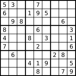
On the left we have a Sudoku puzzle and on the right we see the solution (2).

In Sudoku we need uniqueness along the rows, the columns and inside the 3 x 3 sub-squares. The constraints that enforce these uniqueness conditions are:

\[\boxed{\begin{align}&\sum_j x_{i,j,k} = 1 &&\forall i, k&& \text{value $k$ appears once in row $i$}\\
&\sum_j x_{i,j,k} = 1 &&\forall j, k&& \text{value $k$ appears once in column $j$}\\
&\sum_{i,j|u_{s,i,j}} x_{i,j,k} = 1 &&\forall s, k&& \text{value $k$ appears once in square $s$}\\
                       &\sum_k x_{i,j,k} = 1&&\forall i, j&&\text{cell $(i,j)$ contains one value}
              \end{align}}\]

Here \(u_{s,i,j}\) contains the elements \(i,j\) for square \(s\). With this we have two issues left: How can we build up \(u_{s,i,j}\) and how can we fix the given values in the Sudoku problem.

Populate areas

We number the squares as follows:

image

Let’s see if we can populate \(u_{s,i,j}\) without entering data manually and without using loops. We can invent a function \(s=f(i,j)\) that takes a row and column number and returns the number of the square as follows:

\[f(i,j) = 3\left\lceil i/3 \right\rceil + \left\lceil j/3 \right\rceil – 3\]

Here the funny brackets indicate the ceiling function. E.g. \(f(4,7)= 3\left\lceil 4/3 \right\rceil + \left\lceil 7/3 \right\rceil –3 = 3\cdot 2+3-3=6\). This means we can populate \(u\) as in:

image

When we take a step back, we can consider rows and columns as just another particularly shaped block. So we add to our set \(u\) the individual rows and columns:

image

To verify we get the correct data structure, you may want to display u:

----     23 SET u  areas with unique values

               c1          c2          c3          c4          c5          c6          c7          c8          c9

r1.r1         YES         YES         YES         YES         YES         YES         YES         YES         YES
r2.r2         YES         YES         YES         YES         YES         YES         YES         YES         YES
r3.r3         YES         YES         YES         YES         YES         YES         YES         YES         YES
r4.r4         YES         YES         YES         YES         YES         YES         YES         YES         YES
r5.r5         YES         YES         YES         YES         YES         YES         YES         YES         YES
r6.r6         YES         YES         YES         YES         YES         YES         YES         YES         YES
r7.r7         YES         YES         YES         YES         YES         YES         YES         YES         YES
r8.r8         YES         YES         YES         YES         YES         YES         YES         YES         YES
r9.r9         YES         YES         YES         YES         YES         YES         YES         YES         YES
c1.r1         YES
c1.r2         YES
c1.r3         YES
c1.r4         YES
c1.r5         YES
c1.r6         YES
c1.r7         YES
c1.r8         YES
c1.r9         YES
c2.r1                     YES
c2.r2                     YES
c2.r3                     YES
c2.r4                     YES
c2.r5                     YES
c2.r6                     YES
c2.r7                     YES
c2.r8                     YES
c2.r9                     YES
c3.r1                                 YES
c3.r2                                 YES
c3.r3                                 YES
c3.r4                                 YES
c3.r5                                 YES
c3.r6                                 YES
c3.r7                                 YES
c3.r8                                 YES
c3.r9                                 YES
c4.r1                                             YES
c4.r2                                             YES
c4.r3                                             YES
c4.r4                                             YES
c4.r5                                             YES
c4.r6                                             YES
c4.r7                                             YES
c4.r8                                             YES
c4.r9                                             YES
c5.r1                                                         YES
c5.r2                                                         YES
c5.r3                                                         YES
c5.r4                                                         YES
c5.r5                                                         YES
c5.r6                                                         YES
c5.r7                                                         YES
c5.r8                                                         YES
c5.r9                                                         YES
c6.r1                                                                     YES
c6.r2                                                                     YES
c6.r3                                                                     YES
c6.r4                                                                     YES
c6.r5                                                                     YES
c6.r6                                                                     YES
c6.r7                                                                     YES
c6.r8                                                                     YES
c6.r9                                                                     YES
c7.r1                                                                                 YES
c7.r2                                                                                 YES
c7.r3                                                                                 YES
c7.r4                                                                                 YES
c7.r5                                                                                 YES
c7.r6                                                                                 YES
c7.r7                                                                                 YES
c7.r8                                                                                 YES
c7.r9                                                                                 YES
c8.r1                                                                                             YES
c8.r2                                                                                             YES
c8.r3                                                                                             YES
c8.r4                                                                                             YES
c8.r5                                                                                             YES
c8.r6                                                                                             YES
c8.r7                                                                                             YES
c8.r8                                                                                             YES
c8.r9                                                                                             YES
c9.r1                                                                                                         YES
c9.r2                                                                                                         YES
c9.r3                                                                                                         YES
c9.r4                                                                                                         YES
c9.r5                                                                                                         YES
c9.r6                                                                                                         YES
c9.r7                                                                                                         YES
c9.r8                                                                                                         YES
c9.r9                                                                                                         YES
s1.r1         YES         YES         YES
s1.r2         YES         YES         YES
s1.r3         YES         YES         YES
s2.r1                                             YES         YES         YES
s2.r2                                             YES         YES         YES
s2.r3                                             YES         YES         YES
s3.r1                                                                                 YES         YES         YES
s3.r2                                                                                 YES         YES         YES
s3.r3                                                                                 YES         YES         YES
s4.r4         YES         YES         YES
s4.r5         YES         YES         YES
s4.r6         YES         YES         YES
s5.r4                                             YES         YES         YES
s5.r5                                             YES         YES         YES
s5.r6                                             YES         YES         YES
s6.r4                                                                                 YES         YES         YES
s6.r5                                                                                 YES         YES         YES
s6.r6                                                                                 YES         YES         YES
s7.r7         YES         YES         YES
s7.r8         YES         YES         YES
s7.r9         YES         YES         YES
s8.r7                                             YES         YES         YES
s8.r8                                             YES         YES         YES
s8.r9                                             YES         YES         YES
s9.r7                                                                                 YES         YES         YES
s9.r8                                                                                 YES         YES         YES
s9.r9                                                                                 YES         YES         YES

This means we can reduce the model equations to just:

\[\boxed{\begin{align}&\sum_{i,j|u_{a,i,j}} x_{i,j,k} = 1 &&\forall a, k&& \text{value $k$ appears once in area $a$}\\
                       &\sum_k x_{i,j,k} = 1&&\forall i, j&&\text{cell $(i,j)$ contains one value}\\
                       &x_{i,j,k} \in \{0,1\}
              \end{align}}\]
Fixing initial values

If we use the variables \(v_{i,j}\) in the model, we can use them to fix the initial values.

image

If we don’t have the \(v\) variables in the model we can fix the underlying \(x\) variables:

image

Complete model

image

The input is most conveniently organized as a table:

table v0(i,j)
  
c1 c2 c3 c4 c5 c6 c7 c8 c9

r1  5  3        7
r2  6        1  9  5
r3     9  8              6
r4  8           6           3
r5  4        8     3        1
r6  7           2           6
r7     6              2  8
r8           4  1  9        5
r9              8        7  9

;

The output looks like:

----     49 PARAMETER v 

         c1       c2       c3       c4       c5       c6       c7       c8       c9

r1        5        3        4        6        7        8        9        1        2
r2        6        7        2        1        9        5        3        4        8
r3        1        9        8        3        4        2        5        6        7
r4        8        5        9        7        6        1        4        2        3
r5        4        2        6        8        5        3        7        9        1
r6        7        1        3        9        2        4        8        5        6
r7        9        6        1        5        3        7        2        8        4
r8        2        8        7        4        1        9        6        3        5
r9        3        4        5        2        8        6        1        7        9


KenKen

On the left we have a KenKen puzzle and on the right we see the solution (4).

In the KenKen puzzle we need to have unique values along the rows and the columns. As we have seen in Sudoku example, this is straightforward. We can formulate this as:

\[\boxed{\begin{align}&\sum_j x_{i,j,k} = 1 &&\forall i, k&& \text{value $k$ appears once in row $i$}\\
&\sum_i x_{i,j,k} = 1 &&\forall j, k&& \text{value $k$ appears once in column $j$}\\
&\sum_k x_{i,j,k} = 1&&\forall i, j&&\text{cell $(i,j)$ contains one value}\\

                       &x_{i,j,k} \in \{0,1\}
              \end{align}}\]

As in the Sudoku example, we can combine the first two constraints into a single one:

\[\sum_{i,j|u_{s,i,j}} x_{i,j,k} = 1 \>\>\forall s,k\]
Lemma

In the subsequent discussion we will make use of the following logarithmic transformation:

Given the construct

\[v_{i,j} = \sum_k k \cdot x_{i,j,k}\]

where \(x_{i,j,k}\in \{0,1\}\),  \(k=1,\dots,K\) and \(\displaystyle\sum_k x_{i,j,k}=1\) we have

\[\log(v_{i,j}) = \sum_k \log(k) \cdot x_{i,j,k}\]

In addition to these uniqueness constraints we have a slew of restrictions related to collections of cells - these are called the cages. Each cage has a rule and a given answer. For instance the first cage in the example above with rule 11+ means that the values of the cells in the cage need to add up to 11 (the solution turns out to be 5+6). Let’s discuss them in detail:

  1. n this is a single cell with a given value. This case is not present in the data set in our example above. The rule is easy: just put the number in the cell \((i,j)\): \(v_{i,j} = n\),
    image 
    For this example we would fix this cell to the value 1.
  2. n+ indicates we add up the values in the cage and the result should be n. This is a simple linear constraint: \[\sum_{i,j|C{i,j}} v_{i,j} = n\]
  3. n- is a cage with just two cells where the absolute value difference between the values of the two cells is n. I.e. \[|v_{i_1,j_1}- v_{i_2,j_2}|=n\] In (6) it is proposed to model this in a linear fashion with the help of an additional binary variable as: \[v_{i_1,j_1}- v_{i_2,j_2}=n(2 \delta-1)\] where \(\delta \in \{0,1\}\). 
  4. n* indicates we multiply all values in the cage: \[\prod_{i,j|C{i,j}} v_{i,j} = n\] In (6) a number of possible linearizations are mentioned, some of them rather complicated with such things as prime number factorizations. Let me suggest a much simpler approach using logarithms. We have: \[\begin{align}&\prod_{i,j|C{i,j}} v_{i,j} = n\\ \Longrightarrow\>\> & \sum_{i,j|C_{i,j}} \log(v_{i,j}) = \log(n)\\ \Longrightarrow\>\> & \sum_{i,j|C_{i,j}} \sum_k \log(k) x_{i,j,k} = \log(n)\end{align}\] The last constraint is linear in the decision variables \(x_{i,j,k}\)!. We have used here that \(\log(v_{i,j})=\sum_k \log(k) x_{i,j,k}\). This simpler linearization is not mentioned in (6).
    Note that we can always evaluate \(\log(k)\) and \(\log(n)\) as \(k\ge 1\) and \(n \ge 1\).
  5. this operation has two cells, and indicates division and can be described more formally: \[\frac{v_{i_1,j_1}}{v_{i_2,j_2}}=n \>\text{or}\>\frac{v_{i_2,j_2}}{v_{i_1,j_1}}=n\] In (6) the following linearization is proposed:\[\begin{align} &v_{i_1,j_1}-n\cdot v_{i_2,j_2} \ge 0-M\cdot \delta\\&v_{i_1,j_1}-n\cdot v_{i_2,j_2} \le 0+M\cdot \delta\\&v_{i_2,j_2}-n\cdot v_{i_1,j_1} \ge 0-M\cdot (1-\delta)\\&v_{i_2,j_2}-n\cdot v_{i_1,j_1} \le 0+M\cdot (1-\delta)\\&\delta\in\{0,1\}\end{align}\] Again I would suggest a simpler linearization: \[\begin{align}&\frac{v_{i_1,j_1}}{v_{i_2,j_2}}=n \>\text{or}\>\frac{v_{i_2,j_2}}{v_{i_1,j_1}}=n\\ \Longrightarrow\>\>&\log(v_{i_1,j_1})-\log(v_{i_2,j_2})=\log(n) \> \text{or} \>\log(v_{i_2,j_2})-\log(v_{i_1,j_1})=\log(n)\\ \Longrightarrow\>\>&|\log(v_{i_1,j_1})-\log(v_{i_2,j_2})|=\log(n)\\  \Longrightarrow\>\>&\log(v_{i_1,j_1})-\log(v_{i_2,j_2})=\log(n)(2\delta-1)\\  \Longrightarrow\>\>&\sum_k \log(k) x_{i_1,j_1,k}-\sum_k \log(k) x_{i_2,j_2,k}=\log(n)(2\delta-1)\end{align}\]
    I believe we can assume \(n\ge 1\) even for subtraction, hence we can safely apply the logarithm.
Complete Model

We have now all the pieces to assemble the complete model.

image

The sets are almost identical to the Sudoku model. We have introduced new sets \(op\), \(p\) and \(c\). The unique values will be handled through a set \(u\) as before, only now this set is simpler: only rows and columns (no squares).

We have a somewhat complicated parameter that holds the problem data:

image

The data can be entered as follows:

parameter operation(c,op,i,j) /
 
cage1 .plus.(r1,r2).c1              11
 
cage2 .div .r1.(c2,c3)               2
 
cage3 .min .r2.(c2,c3)               3
 
cage4 .mul .(r1,r2).c4              20
 
cage5 .mul .(r1.c5, (r1,r2,r3).c6)   6
 
cage6 .div .(r2,r3).c5               3
 
cage7 .mul .(r3,r4).(c1,c2)        240
 
cage8 .mul .r3.(c3,c4)               6
 
cage9 .mul .(r4,r5).c3               6
 
cage10.plus.((r4,r5).c4, r5.c5)      7
 
cage11.mul .r4.(c5,c6)              30
 
cage12.mul .r5.(c1,c2)               6
 
cage13.plus.(r5,r6).c6               9
 
cage14.plus.r6.(c1*c3)               8
 
cage15.div .r6.(c4,c5)               2
/
;

We need to extract data from this data structure to make things easier:

image

The sets \(cells\), \(cellp\) and the parameter \(n\) look like:

----     53 SET cells  cells in cage

                   c1          c2          c3          c4          c5          c6

cage1 .r1         YES
cage1 .r2         YES
cage2 .r1                     YES         YES
cage3 .r2                     YES         YES
cage4 .r1                                             YES
cage4 .r2                                             YES
cage5 .r1                                                         YES         YES
cage5 .r2                                                                     YES
cage5 .r3                                                                     YES
cage6 .r2                                                         YES
cage6 .r3                                                         YES
cage7 .r3         YES         YES
cage7 .r4         YES         YES
cage8 .r3                                 YES         YES
cage9 .r4                                 YES
cage9 .r5                                 YES
cage10.r4                                             YES
cage10.r5                                             YES         YES
cage11.r4                                                         YES         YES
cage12.r5         YES         YES
cage13.r5                                                                     YES
cage13.r6                                                                     YES
cage14.r6         YES         YES         YES
cage15.r6                                             YES         YES


----     53 SET cellp  ordered cell numbers

cage1 .p1.r1.c1
cage1 .p2.r2.c1
cage2 .p1.r1.c2
cage2 .p2.r1.c3
cage3 .p1.r2.c2
cage3 .p2.r2.c3
cage4 .p1.r1.c4
cage4 .p2.r2.c4
cage5 .p1.r1.c5
cage5 .p2.r1.c6
cage5 .p3.r2.c6
cage5 .p4.r3.c6
cage6 .p1.r2.c5
cage6 .p2.r3.c5
cage7 .p1.r3.c1
cage7 .p2.r3.c2
cage7 .p3.r4.c1
cage7 .p4.r4.c2
cage8 .p1.r3.c3
cage8 .p2.r3.c4
cage9 .p1.r4.c3
cage9 .p2.r5.c3
cage10.p1.r4.c4
cage10.p2.r5.c4
cage10.p3.r5.c5
cage11.p1.r4.c5
cage11.p2.r4.c6
cage12.p1.r5.c1
cage12.p2.r5.c2
cage13.p1.r5.c6
cage13.p2.r6.c6
cage14.p1.r6.c1
cage14.p2.r6.c2
cage14.p3.r6.c3
cage15.p1.r6.c4
cage15.p2.r6.c5


----     53 PARAMETER n  value for each cage

cage1   11.000,    cage2    2.000,    cage3    3.000,    cage4   20.000,    cage5    6.000,    cage6    3.000
cage7  240.000,    cage8    6.000,    cage9    6.000,    cage10   7.000,    cage11  30.000,    cage12   6.000
cage13   9.000,    cage14   8.000,    cage15   2.000

The variables in the model are as follows:

image

The loop to fix some cells is not used in this data set as we don’t have fixed values in the data. The rest of the model looks like:

image

The summations in the subtraction and divisions are a little bit misleading. These just pick the value of the first (p1) and second (p2) cell in the cage c. In the division equation we pick up the logarithm of the value. Here are the actually generated MIP rows:

---- subtraction  =E=  cages with subtraction

subtraction(cage3)..  v(r2,c2) - v(r2,c3) + 6*delta(cage3) =E= 3 ; (LHS = 0, INFES = 3 ****)
    

---- division  =E=  cages with division

division(cage2)..  logv(r1,c2) - logv(r1,c3) + 1.38629436111989*delta(cage2) =E= 0.693147180559945 ;
    
      (LHS = 0, INFES = 0.693147180559945 ****)
    
division(cage6)..  logv(r2,c5) - logv(r3,c5) + 2.19722457733622*delta(cage6) =E= 1.09861228866811 ;
    
      (LHS = 0, INFES = 1.09861228866811 ****)
    
division(cage15)..  logv(r6,c4) - logv(r6,c5) + 1.38629436111989*delta(cage15) =E= 0.693147180559945 ;
    
      (LHS = 0, INFES = 0.693147180559945 ****)

In equations \(calclogv\) we could restrict the calculation of \(logv\) only for those cells \((i,j)\) where we have a multiplication or division. Similarly, we can calculate \(v_{i,j}\) only for cells where we do addition or subtraction. Now we calculate too many \(logv\)’s and \(v\)'s. For this small case this is not an issue. Furthermore a good LP/MIP presolver will probably detect a variable that is not used anywhere else, and will remove the variable and the accompanying equation. 

The final result looks like:

----    101 VARIABLE v.L  value

            c1          c2          c3          c4          c5          c6

r1       5.000       6.000       3.000       4.000       1.000       2.000
r2       6.000       1.000       4.000       5.000       2.000       3.000
r3       4.000       5.000       2.000       3.000       6.000       1.000
r4       3.000       4.000       1.000       2.000       5.000       6.000
r5       2.000       3.000       6.000       1.000       4.000       5.000
r6       1.000       2.000       5.000       6.000       3.000       4.000

Conclusion

To solve the KenKen puzzle as a Mixed Integer Program, we can start with a data structure similar as used in the Sodoku formulation: \(x_{i,j,k}\in\{0,1\}\). Using different linearizations from the ones shown in (6) we can solve then KenKen problem easily with a MIP solver.

References

  1. All-different and Mixed Integer Programming, http://yetanothermathprogrammingconsultant.blogspot.com/2016/05/all-different-and-mixed-integer.html
  2. Sudoku, https://en.wikipedia.org/wiki/Sudoku
  3. Sudoku Puzzle, http://www.nytimes.com/crosswords/game/sudoku/hard
  4. KenKen, https://en.wikipedia.org/wiki/KenKen
  5. KenKen Puzzle, http://www.nytimes.com/ref/crosswords/kenken.html
  6. Vardges Melkonian, “An Integer Programming Model for the KenKen Problem”, American Journal of Operations Research, 2016, 6, 213-225. [link] Contains a complete AMPL model.
  7. Andrew C. Bartlett, Timothy P. Chartier, Amy N. Langville, Timothy D. Rankin, “An Integer Programming Model for the Sudoku Problem”, The Journal of Online Mathematics and Its Applications, Vol.8, 2008, [link]