Who needs Cplex or Gurobi: solving LPs using LU

The strange notion that linear programming problems can be solved simply by applying an LU decomposition (not as part of the Simplex method but just LU) seems to take hold. The original idea is from (1) but now we also can use LU as a solver for “Fuzzy Linear Fractional Programming Problems” (2).

 

I agree with the abstract: the proposed approach is simple.

References

1. S.M.Chincole, A.P.Bhadane, LU Factorization Method To Solve Linear Programming Problem, International Journal of Emerging Technology and Advanced Engineering ,Volume 4, Issue 4, 176-180, http://www.ijetae.com/files/Volume4Issue4/IJETAE_0414_31.pdf. Warning: this method does not work except in some very special cases (e.g. all constraints binding in the optimal solution).
2. S. Muruganandam and P. Ambika,  Solving Fuzzy Linear Fractional Programming Problem using LU Decomposition Method, Annals of Pure and Applied Mathematics, Vol. 13, No 1., 2017, pp 89-97.
3. Solving LP by LU??, http://yetanothermathprogrammingconsultant.blogspot.com/2017/01/solving-lp-by-lu.html

Minimizing the k-th largest x

Minimizing the largest $x_i$ is an easy exercise in LP modeling:

$$\bbox[lightcyan,10px,border:3px solid darkblue] { \begin{align} \min\>& z\\ & z \ge x_i \end{align}}$$

This is sometimes called MINIMAX.

What about minimizing the $k^{\text{th}}$ largest value? Here is one possible MIP formulation:

$$\bbox[lightcyan,10px,border:3px solid darkblue] { \begin{align} \min\>& z\\ & z \ge x_i - \delta_i M\\ & \sum_i \delta_i = k-1\\ & \delta_i \in \{0,1\} \end{align}}$$

I.e., we have $k-1$ exceptions on the constraint $z \ge x_i$. The objective will make sure the exceptions are the largest $x_i$.  We should think long and hard about making the big-M’s as small as possible. If you have no clue about proper bounds on $x_i$ one could use indicator constraints.

Interestingly, minimizing the sum of the $k$ largest can be modeled as a pure LP (1) :

$$\bbox[lightcyan,10px,border:3px solid darkblue] { \begin{align} \min\>& \sum_i v_i + k\cdot q\\ & v_i \ge x_i - q\\ &v_i \ge 0 \\ &q \text{ free } \end{align}}$$

You almost would think there is an LP formulation for minimizing the $k^{\text{th}}$ largest value. I don't see it however.

References

1. Comment by Michael Grant in http://orinanobworld.blogspot.se/2015/08/optimizingpartoftheobjectivefunction-ii.html.

Modeling production runs with length exactly three

In (1) the question was posed how to model production runs that have an exact length. Although the question was asked in terms of integer variables, this is much easier to deal with when we have binary variables. Let’s introduce a binary variable:

$$x_{t} = \begin{cases}1 & \text{when the unit $x$ is turned on in period $t$}\\0 &\text{otherwise}\end{cases}$$

The question was formulated as an implication:

$$x_t=1 \implies x_{t+1}=x_{t+2}=1$$

This implication is not 100% correct: it would turn on $x$ forever. But we understand what the poster meant, if a unit is turned on, it should stay on for exactly three periods.

This condition can be more correctly stated as the implication:

$$x_{t-1}=0 \text{ and } x_{t}=1 \implies x_{t+1}=x_{t+2}=1 \text{ and } x_{t+3}=0$$

We can make linear inequalities out of this as follows:

$$\bbox[lightcyan,10px,border:3px solid darkblue]{\begin{align}&x_{t+1}\ge x_{t}-x_{t-1}\\&x_{t+2}\ge x_{t}-x_{t-1}\\&1-x_{t+3}\ge x_{t}-x_{t-1}\end{align}}$$

If we want to model the condition “a unit should stay on for at least three periods”, we can drop the last constraint and just keep:

$$\begin{align}&x_{t+1}\ge x_{t}-x_{t-1}\\&x_{t+2}\ge x_{t}-x_{t-1}\end{align}$$

References

1. https://stackoverflow.com/questions/44496473/block-of-consecutive-variables-to-have-same-value-in-mixed-integer-linear-progra

A Staffing Problem

In (1) a "simple problem" is stated (problems are rarely as simple as they seem):

For the next 18 weeks there is some data about demand for staffing resources:

Actually we don’t need the data for the individual projects: just the totals. It is noted that the maximum number of “bodies” we need is 52 (in week 3).

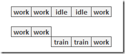
We start with 48 temps available in the first period. We can let a temp staffer go and we can hire new ones. However when hiring a staffer it will cost 10 days (2 weeks) to train this person. During training a staffer is not productive.  We can also keep a staffer idling for a few periods.

To make a difference between idling and training, as shown here:

I will assume that hiring + training is slightly more expensive than keeping someone idle. I think it makes sense to assign some cost to the hiring and training process. This property was not in the original post but I think I have convinced myself that this is actually a reasonable assumption.

To model this I introduce two sets of binary variables:

$$\begin{align} & r_{i,t} = \begin{cases} 1 & \text{if a staffer $i$ is available for training or work during period $t$}\\ 0 & \text{otherwise} \end{cases} \\ & h_{i,t} = \begin{cases} 1 & \text{if a staffer $i$ is hired at the beginning of period $t$}\\ 0 & \text{otherwise} \end{cases} \end{align}$$

We can link $h_{i,t}$ and $r_{i,t}$ as follows:

$$h_{i,t}\ge r_{i,t}-r_{i,t-1}$$

This implements the implication:

$$r_{i,t-1}=0 \text{ and } r_{i,t}=1 \implies h_{i,t}=1$$

that is: if we change $r$ from 0 to 1, we have a new hire. We will add a (small) cost to a hire to the objective so we don’t need to add constraint to enforce the other way around:

$$r_{i,t-1}=1 \text{ or } r_{i,t}=0 \implies h_{i,t}=0$$

There is one wrinkle here: we need to make sure that the 48 staffers already hired before can work in the first period without being considered to be hired. We can explicitly model this:

$$h_{i,t}\ge \begin{cases} r_{i,t}-r_{i,t-1} &\text{if $t>1$}\\ r_{i,t}&\text{if $t=1$ and $i>48$}\end{cases}$$

Actually in the GAMS model below I approached this slightly differently, but with the same net result.

The main equation in the model is to make sure we have enough staffing in each period $t$. This can be modeled as:

$$\sum_i \left( r_{i,t} – h_{i,t} - h_{i,t-1}\right) \ge \mathit{demand}_t$$

The complete model can look like:

Notes:

• $\mathit{rinit}_{i,t}$ is used to indicate initial staffing when we start period 1. It is sparse: it assumes the value 1 only if $i=1$ and $t \le 48$.
• This allows us to write equation EHire as one single, clean equation.
• Note that GAMS will assume a variable is zero outside its domain:  $r_{i,t-1}$ is zero when $t=1$.
• I used the maximum demand (52 in week 3) to dimension the the problem: set $i$ has 52 members.
• The model does not decide which workers are idle. We can see in each period how many workers we have and how many are in training. The remaining ones are working or sitting idle.
• We reuse resource numbers $i$. In the results below worker $i=21$ is likely to be two different persons.

The results look like:

 

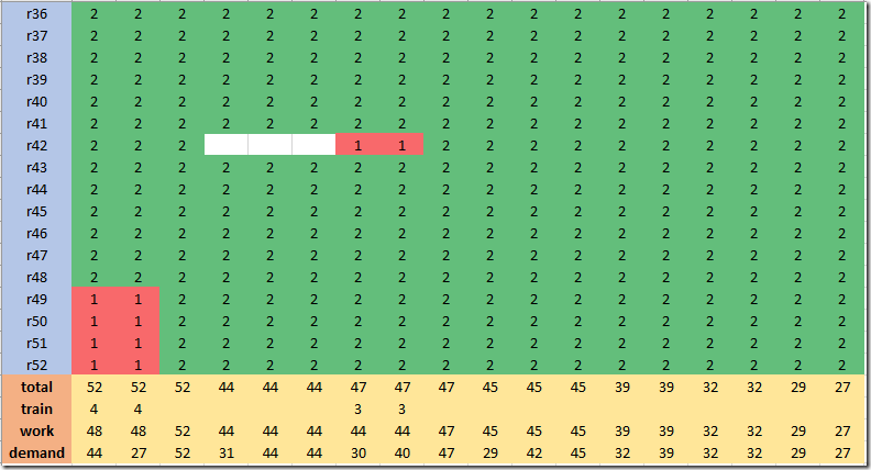
Here a green cell with code=2 means hired and working (or idle, but not in training). A red cell with code=1 means in training.  The row “total” is the number of staffers (either working, idling or training). The row “Work” indicates the number of workers available (not in training). We are overshooting demand a bit: some workers are idling.

A picture is always a good idea, so here we see demand vs. staffing available for work.

We see two place where we increase the workforce: we hire in week 1 to handle demand in week 3, and we hire again in week 7 to deal with demand in week 9.

References

• Resources Management Linear Programming, https://stackoverflow.com/questions/44402163/resources-management-linear-programming

Minimum down- and up-time

In machine scheduling models we sometimes want to impose minimum up-time and minimum down-time restrictions. E.g., from (1):

My question is how do I add in additional constraints that if the factory switches off then its needs to stay off for 3 months, and if it switches back on then it needs to stay on for 4 months?

One possible solution is the following. Let us define our binary decision variable by

$$x_{i,t} = \begin{cases}1 & \text{if factory $i$ is operating in month $t$} \\   0&\text{otherwise} \end{cases}$$

Method 1

We really want to forbid short run patterns such as 010 (i.e. off-on-off), 0110, 01110 and 101, 1001. Forbidding patterns 010, 0110, 01110 will ensure a factory is up at least 4 consecutive periods. By not allowing 101,1001 we really make sure that a down time period is at least three months. We can model these restrictions in a linear fashion as follows (2):

Forbid 010	$-x_{i,t}+x_{i,t+1}-x_{i,t+2}\le 0$
Forbid 0110	$-x_{i,t}+x_{i,t+1}+x_{i,t+2}-x_{i,t+3}\le 1$
Forbid 01110	$-x_{i,t}+x_{i,t+1}+x_{i,t+2}+x_{i,t+3}-x_{i,t+4}\le 2$
Forbid 101	$x_{i,t}-x_{i,t+1}+x_{i,t+2}\le 1$
Forbid 1001	$x_{i,t}-x_{i,t+1}-x_{i,t+2}+x_{i,t+3}\le 1$

Method 2

A different approach is as follows. First define binary variables:

$$\begin{align} &\delta^{\mathit{on}}_{i,t} = \begin{cases}1 & \text{if factory $i$ is turned on in month $t$} \\   0&\text{otherwise} \end{cases}\\ &\delta^{\mathit{off}}_{i,t} = \begin{cases}1 & \text{if factory $i$ is turned off in month $t$} \\   0&\text{otherwise} \end{cases} \end{align}$$

Mathematically we write this as:

$$\begin{align} &\delta^{\mathit{on}}_{i,t} = (1-x_{i,t-1})\cdot x_{i,t}\\ &\delta^{\mathit{off}}_{i,t} = x_{i,t-1}\cdot (1-x_{i,t})\\ \end{align}$$

We can linearize these non-linear equations by:

$$\begin{align} &\delta^{\mathit{on}}_{i,t} \le 1-x_{i,t-1}\\ &\delta^{\mathit{on}}_{i,t} \le x_{i,t}\\ &\delta^{\mathit{on}}_{i,t} \ge x_{i,t}-x_{i,t-1}\\ &\delta^{\mathit{off}}_{i,t} \le x_{i,t-1}\\ &\delta^{\mathit{off}}_{i,t} \le 1-x_{i,t}\\ &\delta^{\mathit{off}}_{i,t} \ge x_{i,t-1}-x_{i,t}\\ \end{align}$$

With these variables we can implement the implications:

$$\begin{align} &\delta^{\mathit{on}}_{i,t} = 1 \implies x_{i,t} + x_{i,t+1} + x_{i,t+2} + x_{i,t+3} = 4 \\ &\delta^{\mathit{off}}_{i,t} = 1 \implies x_{i,t} + x_{i,t+1} + x_{i,t+2} = 0 \end{align}$$

This can be linearized as:

$$\begin{align} & x_{i,t+1} + x_{i,t+2} + x_{i,t+3} \ge 3 \delta^{\mathit{on}}_{i,t} \\ & x_{i,t+1} + x_{i,t+2} \le 2 (1-\delta^{\mathit{off}}_{i,t}) \end{align}$$

Note that I dropped $x_{i,t}$ in both inequalities. These are already known from the definition of $\delta^{\mathit{on}}_{i,t}$ and $\delta^{\mathit{off}}_{i,t}$.

In the comments it is mentioned by Rob Pratt that we can strengthen this a bit (the math does not look very good in a comment, so I repeat it here):

$$\begin{align} & x_{i,t+1} \ge \delta^{\mathit{on}}_{i,t}\\ & x_{i,t+2} \ge \delta^{\mathit{on}}_{i,t}\\ & x_{i,t+3} \ge \delta^{\mathit{on}}_{i,t}\\ & x_{i,t+1} \le 1-\delta^{\mathit{off}}_{i,t} \\ & x_{i,t+2} \le 1-\delta^{\mathit{off}}_{i,t} \end{align}$$

References

1. How do I add a constraint to keep a factory switched on or off for a certain period of time in PuLP? https://stackoverflow.com/questions/44281389/how-do-i-add-a-constraint-to-keep-a-factory-switched-on-or-off-for-a-certain-per/44293592
2. Integer cuts, http://yetanothermathprogrammingconsultant.blogspot.com/2011/10/integer-cuts.html

References

Wednesday, June 7, 2017