On the scheduling of reading book chapters

In [1] an interesting problem is posted:

I want to read a book in a given number of days.  I want to read an integer number of chapters each day (there are more chapters than days), no stopping part way through a chapter, and at least 1 chapter each day.  The chapters are very non uniform in length (some very short, a few very long, many in between) so I would like to come up with a reading schedule that minimizes the variance of the length of the days readings (read multiple short chapters on the same day, long chapters are the only one read that day).  I also want to read through the book in order (no skipping ahead to combine short chapters that are not naturally next to each other. 

The data set is the Book of Mormons [2]:

Chapter	Words	Letters	Verses	Chapter	Words	Letters	Verses
1 Nephi 1	908	3746	20	Alma 26	1665	6840	37
1 Nephi 2	879	3640	24	Alma 27	1260	5294	30
1 Nephi 3	1067	4295	31	Alma 28	575	2471	14
1 Nephi 4	1262	4968	38	Alma 29	708	2748	17
1 Nephi 5	761	3202	22	Alma 30	2666	10762	60
1 Nephi 6	202	777	6	Alma 31	1478	6269	38
1 Nephi 7	992	3941	22	Alma 32	1837	7479	43
1 Nephi 8	1221	4769	38	Alma 33	855	3416	23
1 Nephi 9	259	1075	6	Alma 34	1576	6477	41
1 Nephi 10	924	3829	22	Alma 35	699	3043	16
1 Nephi 11	1315	5159	36	Alma 36	1229	4719	30
1 Nephi 12	860	3527	23	Alma 37	2027	8764	47
1 Nephi 13	1899	7874	42	Alma 38	651	2494	15
1 Nephi 14	1284	5236	30	Alma 39	793	3168	19
1 Nephi 15	1488	6149	36	Alma 40	1153	4790	26
1 Nephi 16	1618	6555	39	Alma 41	701	2983	15
1 Nephi 17	2523	10180	55	Alma 42	1229	5129	31
1 Nephi 18	1217	4960	25	Alma 43	2221	9795	54
1 Nephi 19	1292	5399	24	Alma 44	1243	5043	24
1 Nephi 20	698	2767	22	Alma 45	911	3913	24
1 Nephi 21	945	3758	26	Alma 46	1809	7635	41
1 Nephi 22	1506	6275	31	Alma 47	1572	6693	36
2 Nephi 1	1543	6391	32	Alma 48	1073	4669	25
2 Nephi 2	1460	6151	30	Alma 49	1345	5968	30
2 Nephi 3	1170	4685	25	Alma 50	1734	7508	40
2 Nephi 4	1300	5267	35	Alma 51	1682	7271	37
2 Nephi 5	1169	4767	34	Alma 52	1757	7543	40
2 Nephi 6	895	3780	18	Alma 53	1085	4730	23
2 Nephi 7	405	1574	11	Alma 54	988	4095	24
2 Nephi 8	812	3261	25	Alma 55	1218	5152	35
2 Nephi 9	2388	9985	54	Alma 56	2177	9129	57
2 Nephi 10	966	4106	25	Alma 57	1517	6395	36
2 Nephi 11	338	1332	8	Alma 58	1748	7357	41
2 Nephi 12	647	2557	22	Alma 59	489	2166	13
2 Nephi 13	587	2454	26	Alma 60	1777	7512	36
2 Nephi 14	203	810	6	Alma 61	854	3544	21
2 Nephi 15	857	3540	30	Alma 62	2220	9554	52
2 Nephi 16	370	1406	13	Alma 63	593	2505	17
2 Nephi 17	687	2668	25	Helaman 1	1418	6171	34
2 Nephi 18	570	2304	22	Helaman 2	599	2568	14
2 Nephi 19	587	2474	21	Helaman 3	1527	6542	37
2 Nephi 20	928	3715	34	Helaman 4	1076	4781	26
2 Nephi 21	520	2090	16	Helaman 5	2084	8655	52
2 Nephi 22	134	533	6	Helaman 6	1797	7721	41
2 Nephi 23	587	2442	22	Helaman 7	1142	4751	29
2 Nephi 24	891	3587	32	Helaman 8	1210	5134	28
2 Nephi 25	1699	7294	30	Helaman 9	1480	6032	41
2 Nephi 26	1483	6363	33	Helaman 10	720	3013	19
2 Nephi 27	1461	5809	35	Helaman 11	1561	6536	38
2 Nephi 28	1240	4997	32	Helaman 12	873	3504	26
2 Nephi 29	804	3197	14	Helaman 13	1855	7527	39
2 Nephi 30	708	2941	18	Helaman 14	1241	5106	31
2 Nephi 31	988	4065	21	Helaman 15	824	3607	17
2 Nephi 32	426	1743	9	Helaman 16	1025	4247	25
2 Nephi 33	647	2539	15	3 Nephi 1	1340	5524	30
Jacob 1	719	3149	19	3 Nephi 2	769	3404	19
Jacob 2	1365	5815	35	3 Nephi 3	1353	5947	26
Jacob 3	619	2765	14	3 Nephi 4	1518	6506	33
Jacob 4	929	4027	18	3 Nephi 5	931	3891	26
Jacob 5	3758	15366	77	3 Nephi 6	1200	5256	30
Jacob 6	511	2091	13	3 Nephi 7	1132	4944	26
Jacob 7	1242	4988	27	3 Nephi 8	871	3700	25
Enos 1	1160	4730	27	3 Nephi 9	965	4006	22
Jarom 1	734	3149	15	3 Nephi 10	807	3392	19
Omni 1	1398	5906	30	3 Nephi 11	1434	5732	41
Words of Mormon 1	857	3704	18	3 Nephi 12	1294	5185	48
Mosiah 1	966	4188	18	3 Nephi 13	834	3402	34
Mosiah 2	2112	8675	41	3 Nephi 14	628	2451	27
Mosiah 3	1117	4771	27	3 Nephi 15	731	2962	24
Mosiah 4	1605	6586	30	3 Nephi 16	913	3679	20
Mosiah 5	740	2965	15	3 Nephi 17	879	3550	25
Mosiah 6	309	1313	7	3 Nephi 18	1344	5429	39
Mosiah 7	1555	6326	33	3 Nephi 19	1233	5083	36
Mosiah 8	938	3948	21	3 Nephi 20	1538	6354	46
Mosiah 9	864	3489	19	3 Nephi 21	1155	4659	29
Mosiah 10	957	3942	22	3 Nephi 22	507	2155	17
Mosiah 11	1271	5205	29	3 Nephi 23	415	1754	14
Mosiah 12	1291	5309	37	3 Nephi 24	620	2496	18
Mosiah 13	1073	4300	35	3 Nephi 25	183	721	6
Mosiah 14	391	1574	12	3 Nephi 26	793	3326	21
Mosiah 15	1056	4559	31	3 Nephi 27	1269	4917	33
Mosiah 16	560	2393	15	3 Nephi 28	1457	5856	39
Mosiah 17	650	2655	20	3 Nephi 29	394	1589	9
Mosiah 18	1382	5755	35	3 Nephi 30	130	564	2
Mosiah 19	978	4070	29	4 Nephi 1	1949	8300	49
Mosiah 20	963	4027	26	Mormon 1	706	2987	19
Mosiah 21	1328	5649	36	Mormon 2	1262	5317	29
Mosiah 22	620	2651	16	Mormon 3	939	3820	22
Mosiah 23	1186	4978	39	Mormon 4	822	3595	23
Mosiah 24	954	3970	25	Mormon 5	1067	4483	24
Mosiah 25	837	3610	24	Mormon 6	914	3664	22
Mosiah 26	1200	5112	39	Mormon 7	454	1805	10
Mosiah 27	1601	6733	37	Mormon 8	1710	6931	41
Mosiah 28	812	3513	20	Mormon 9	1510	6225	37
Mosiah 29	1879	7990	47	Ether 1	901	3508	43
Alma 1	1496	6356	33	Ether 2	1370	5481	25
Alma 2	1433	6179	38	Ether 3	1253	5007	28
Alma 3	1016	4340	27	Ether 4	892	3623	19
Alma 4	1035	4432	20	Ether 5	226	891	6
Alma 5	2787	11260	62	Ether 6	1048	4265	30
Alma 6	390	1657	8	Ether 7	899	3746	27
Alma 7	1443	5913	27	Ether 8	1231	5041	26
Alma 8	1231	5033	32	Ether 9	1424	5823	35
Alma 9	1511	6274	34	Ether 10	1415	5726	34
Alma 10	1442	5835	32	Ether 11	762	3238	23
Alma 11	1466	5865	46	Ether 12	1536	6443	41
Alma 12	1858	7802	37	Ether 13	1219	5053	31
Alma 13	1347	5776	31	Ether 14	1132	4664	31
Alma 14	1526	6295	29	Ether 15	1314	5370	34
Alma 15	711	3034	19	Moroni 1	147	614	4
Alma 16	1010	4383	21	Moroni 2	119	459	3
Alma 17	1848	7842	39	Moroni 3	120	491	4
Alma 18	1623	6659	43	Moroni 4	153	629	3
Alma 19	1701	6905	36	Moroni 5	91	351	2
Alma 20	1279	5104	30	Moroni 6	335	1457	9
Alma 21	955	4162	23	Moroni 7	1929	7812	48
Alma 22	1871	7733	35	Moroni 8	1064	4677	30
Alma 23	764	3321	18	Moroni 9	1012	4305	26
Alma 24	1509	6241	30	Moroni 10	1149	4603	34
Alma 25	752	3212	17

Some additional data:

• The number of days available is \(T=128\).
• The number of chapters to read is \(n=239\). 
• We can minimize the variance of any of the quantities verses, words or letters. Here I use verses.
• The total number of verses is \(\sum_i v_i = 6603\). 
• The average number of verses we want read per day is:\[\mu = \frac{\sum_i v_i}{T}= 51.6\]
• I add the constraint we want to read at least one chapter per day.
• We define the objective to minimize as: \[\min z=\sum_t (nv_t-\mu)^2\] where \(nv_t\) is the number of verses we read during day \(t\).

This is not a very small problem.

Method 1: Dynamic Programming

A dynamic programming approach is found in an answer provided in [1]. Let:

\(f_{i,t} = \) SSQ of optimal schedule when reading chapters \(1,\dots,i\) in \(t\) days.

where SSQ means sum of squares objective. This leads to the recursion:

\[\bbox[lightcyan,10px,border:3px solid darkblue]{\large{f_{i,t} = \min_{k=t-1,\dots,i-1}  \left\{ f_{k,t-1} + \left( \sum_{j=k+1}^i v_j - \mu\right)^2 \right\} }}\]

Now we just need to evaluate \(f_{n,T}\). 

The R code in [1] looks like:

f<-function(X=bom3$Verses,days=128){ 
# find optimal BOM reading schedule for Greg Snow 
# minimize variance of quantity to read per day over 128 days 
# 
N = length(X) 
SSQ<- matrix(NA,nrow=days,ncol=N) 
Cuts <- list() 
# 
#  SSQ[i,j]: the ssqs about the overall mean for the optimal partition 
#           for i days on the chapters 1 to j 
# 
M <- sum(X)/days 
SSQ[1,] <- (cumsum(X)-M)^2 
Cuts[[1]] <- as.list(1:N) 

for (m in 2:days){ 
   Cuts[[m]]=list() 
   for (n in m:N){ 
       CS = cumsum(X[n:1])[n:1] 
       SSQ1 = (CS-M)^2 
       j = (m-1):(n-1) 
       TS = SSQ[m-1,j]+(SSQ1[j+1]) 
       SSQ[m,n] = min(TS) 
       k = min(which((min(TS)== TS)))+m-1 
       Cuts[[m]][[n]] = c(Cuts[[m-1]][[k-1]],n) 
   } 
} 
list(SSQ=SSQ[days,N],Cuts=Cuts[[days]][[N]]) 
} 

This runs very fast:

> library(tictoc)
> tic()
> f()
$SSQ
[1] 11241.05

$Cuts
  [1]   2   4   7   9  11  13  15  16  17  19  21  23  25  27  30  31  34  37  39  41  44  46  48  50
 [25]  53  56  59  60  62  64  66  68  70  73  75  77  78  80  82  84  86  88  89  91  92  94  95  96
 [49]  97  99 100 103 105 106 108 110 112 113 115 117 119 121 124 125 126 127 129 131 132 135 137 138
 [73] 140 141 142 144 145 146 148 150 151 152 154 156 157 160 162 163 164 166 167 169 171 173 175 177
 [97] 179 181 183 185 186 188 190 192 193 194 196 199 201 204 205 207 209 211 213 214 215 217 220 222
[121] 223 225 226 228 234 236 238 239

> toc()
1.08 sec elapsed
> 

To see how we can interpret the solution, let's reproduce the objective function value:

> Days <- 128
> mu <- sum(bom3$Verses)/Days 
> 
> results <- f()
> start <- c(1, head(results$Cuts,-1)+1)
> end <- results$Cuts
> 
> verses <- rep(0,Days)
> for (i in 1:Days) {
+    verses[i] <- sum(v[start[i]:end[i]])
+ }
> 
> sum( (verses-mu)^2 )
[1] 11241.05

Method 2: A nonlinear Assignment Problem formulation

If we define binary variables:\[x_{i,t} = \begin{cases} 1 & \text{if chapter $i$ is read during day $t$}\\ 0 &\text{otherwise}\end{cases}\] we basically have an assignment problem. On top of this we add some ordering constraints and a nonlinear objective that measures the variance in the number of verses read.

The model can look like:

\[\bbox[lightcyan,10px,border:3px solid darkblue]{\begin{align} \min&\sum_t \left(nv_t - \mu\right)^2\\ &\sum_t x_{i,t} = 1 && \forall i\\ &\sum_i x_{i,t} \ge 1 && \forall t \\& x_{i,t} = 1 \Rightarrow x_{i+1,t} + x_{i+1,t+1}=1\\ &nv_t = \sum_i x_{i,t} v_i\\ & x_{1,1} = x_{n,T} = 1\\ & x_{i,t} \in \{0,1\}  \end{align} }\]

Besides assigning each chapter to a day, we need to establish the ordering:

A proper schedule

First we note that we know that the first chapter is read in the first day and the last chapter is read in the last day. This is modeled by fixing \(x_{1,1} = x_{n,T} = 1\). Secondly we have the rule that if \(x_{i,t}=1\) (i.e. chapter \(i\) is read during day \(t\)), then we know that the next chapter \(i+1\) is read during the same day or the next day. This constraint will ensure we build a proper schedule. Formally: \(x_{i,t} = 1 \Rightarrow x_{i+1,t} + x_{i+1,t+1}=1\). The implication can be linearized as: \[ x_{i,t} \le x_{i+1,t} + x_{i+1,t+1} \le 2-x_{i,t}\]
Looking at the allowed patterns, we can actually strengthen this to:
\[ x_{i,t} \le x_{i+1,t} + x_{i+1,t+1} \le 1\]

(this does not seem to help).

This MIQP model is very difficult to solve even with the best available solvers. One of the reasons is that the model is very large: it contains 30,592 binary variables. I am sorry to say this formulation is not very useful. Too bad: I think this formulation has a few interesting wrinkles.

Method 3: A Set Covering Approach

We can look at the problem in a different way. Let

\[x_{i,j} = \begin{cases} 1 & \text{if we read chapters $i$ through $j$}\\ 0 & \text{otherwise} \end{cases}\]

Of course we have \(i \le j \le n\). A set covering type of model can look like:

\[\bbox[lightcyan,10px,border:3px solid darkblue]{\begin{align}\min & \sum_{j\ge i} c_{i,j} x_{i,j}\\ &   \sum_{i \le k \le j} x_{i,j} = 1 && \forall k\\ & \sum_{j\ge i} x_{i,j} = T\\ & x_{i,j} \in \{0,1\}\end{align}}\]

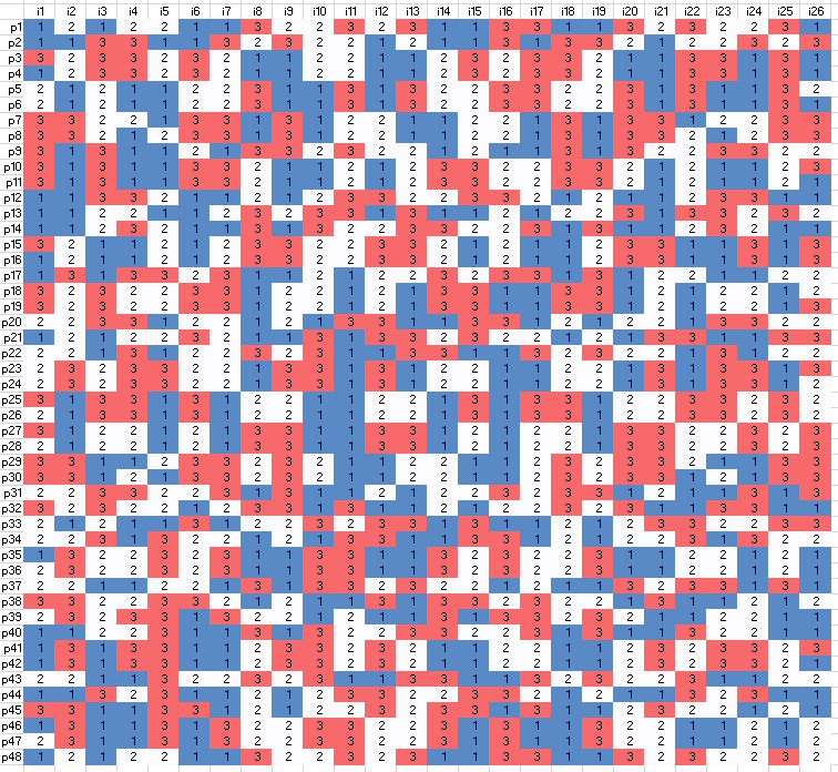
Basically we do the following:

Covering

Select \(T\) variables \(x_{i,j}\) such that each chapter is covered exactly once. In the picture above: select \(T\) rows such that each column is covered by exactly one blue cell. On the right we see a feasible solution for \(T=3\) days. The constraint \(\sum_{i \le k \le j} x_{i,j} = 1, \forall k\) counts the number of ones in a column: it should be exactly one. The constraint \(\sum_{j\ge i} x_{i,j} = T\) selects \(T\) variables.

We can slightly optimize things by noting that we can not read more than  \(n-T+1\) chapters in a single day. We would finish the book too quickly. Remember, we want to read at least a single chapter each day. So, in advance, we can remove from the problem all variables with more than \(n-T+1\) chapters.

Before and after preprocessing

In the picture above we have \(n=4\) and \(T=3\). We can remove all \(x_{i,j}\)'s with length three and longer.

This is now a linear model with binary variables! The variables deal with a whole day, so the quadratic cost is now linear in the decision variables.  It turns out to be not a very difficult MIP:

Iteration log . . .
Iteration:     1   Dual objective     =          2476.602417
Root relaxation solution time = 0.36 sec. (126.25 ticks)

        Nodes                                         Cuts/
   Node  Left     Objective  IInf  Best Integer    Best Bound    ItCnt     Gap

*     0+    0                       134595.0547        0.0000           100.00%
Found incumbent of value 134595.054688 after 9.50 sec. (3892.85 ticks)
*     0     0      integral     0    11241.0547    11241.0547      180    0.00%
Elapsed time = 9.52 sec. (3899.95 ticks, tree = 0.00 MB, solutions = 2)
Found incumbent of value 11241.054688 after 9.52 sec. (3899.95 ticks)

Root node processing (before b&c):
  Real time             =    9.53 sec. (3900.78 ticks)
Sequential b&c:
  Real time             =    0.00 sec. (0.00 ticks)
                          ------------
Total (root+branch&cut) =    9.53 sec. (3900.78 ticks)
MIP status(101): integer optimal solution
Cplex Time: 9.53sec (det. 3900.84 ticks)

Not bad, but slower than the Dynamic Programming method.

Note that our optimization: remove all variables \(x_{i,j}\) with number of chapters exceeding \(n-T+1\) really helps:

Model	Constraints	Variables	Solution time
Original	240	28,680	30 seconds
Optimized	240	20,552	10 seconds

The presolver does not detect this, so we need to preprocess the problem ourselves.

This model has also a very large number of binary variables, but performs infinitely much better than the previous model. One more indication that just counting variables is not a good measure for difficulty.

Method 4: A Network Model

We can look at this problem as a network [3]:

• The nodes are formed by the chapters plus a sink node. So we have \(n+1\) nodes.
• The arcs \((i,j)\) are interpreted as follows: we have a link \((i,j)\) if we start reading at chapter \(i\) and stop at chapter \(j-1\). I.e. arcs only exist for \(j\gt i\).
• In addition we have arcs \((i,\mathit{sink})\). These arcs correspond to reading all remaining chapters starting at \(i\).
• Each arc \((i,j)\) has a cost \(c_{i,j}\) where \[c_{i,j} = \sum_{k=i}^{j-1} \left(v_k - \mu\right)^2\] The sink can be thought of being chapter \(n+1\).

An example with four chapters can look like:

Network Representation

Along the arcs we see which chapters are read. Note there are only forward arcs in this network. 

The idea is to solve this as a shortest path problem from "ch1" to "sink" under the condition that we visit \(T\) "blue" nodes. A standard shortest path is easily formulated as an LP [4]:

\[\begin{align} \min&\sum_{(i,j)\in A} c_{i,j} x_{i,j}\\ & \sum_{(j,i)\in A} x_{j,i} + b_i = \sum_{(i,j)\in A} x_{i,j} && \forall i\\ &x_{i,j} \ge 0 \end{align}\]

where \[b_i = \begin{cases} 1 &\text{if $i=\mathit{ch1}$}\\  -1 & \text{if $i=\mathit{sink}$}\\  0 & \text{otherwise} \end{cases}\]

To make sure we visit \(T\) nodes we split the node balance equation.

\[\bbox[lightcyan,10px,border:3px solid darkblue]{\begin{align} \min&\sum_{(i,j)\in A} c_{i,j} x_{i,j}\\ & \sum_{(j,i)\in A} x_{j,i} + b_i = y_i && \forall i\\ & y_i = \sum_{(i,j)\in A} x_{i,j} && \forall i\\ & \sum_i y_i = T \\ &x_{i,j}, y_i \ge 0 \end{align}}\]

Here \(y_i\) measures the total flow leaving node \(i\) for consumption by other nodes. The set \(A\) is the set of arcs. Again this is now a completely linear model. This model also seems to give integer solutions automatically, so we don't need to use a MIP solver. (Not exactly sure why; I expected we destroyed enough of the network structure this would no longer be the case. To be on the safe side we can solve this as a MIP of course.). The LP model solves very fast:

Tried aggregator 1 time.
LP Presolve eliminated 3 rows and 3 columns.
Aggregator did 2 substitutions.
Reduced LP has 477 rows, 28916 columns, and 58070 nonzeros.
Presolve time = 0.06 sec. (13.96 ticks)
Initializing dual steep norms . . .

Iteration log . . .
Iteration:     1   Dual objective     =          2509.398865
Iteration:   150   Dual objective     =          9379.320313
LP status(1): optimal
Cplex Time: 0.11sec (det. 35.60 ticks)

Optimal solution found.
Objective :       11241.054688

Finally, this version beats the Dynamic Programming algorithm.

We can do slightly better by using the same optimization as in the set covering approach: ignore all \(x_{i,j}\) that correspond to reading more chapters than \(n-T+1\). This leads to a minor improvement in performance:

Tried aggregator 1 time.
LP Presolve eliminated 3 rows and 3 columns.
Aggregator did 2 substitutions.
Reduced LP has 477 rows, 20788 columns, and 41814 nonzeros.
Presolve time = 0.05 sec. (10.07 ticks)
Initializing dual steep norms . . .

Iteration log . . .
Iteration:     1   Dual objective     =          2580.195313
Iteration:   133   Dual objective     =          8804.367188
LP status(1): optimal
Cplex Time: 0.08sec (det. 24.21 ticks)

Optimal solution found.
Objective :       11241.054688

Conclusion

There is more than one way to skin a cat. These are four very different ways to optimize the reading schedule. If a certain model does not work very well, it makes sense to take a step back and see if you can develop something very different.

Resulting schedule

Day	Chapters	Verses	Cost
Day 1	1 Nephi 1, 1 Nephi 2	44	57.5464
Day 2	1 Nephi 3, 1 Nephi 4	69	303.2496
Day 3	1 Nephi 5, 1 Nephi 6, 1 Nephi 7	50	2.5152
Day 4	1 Nephi 8, 1 Nephi 9	44	57.5464
Day 5	1 Nephi 10, 1 Nephi 11	58	41.1402
Day 6	1 Nephi 12, 1 Nephi 13	65	179.9371
Day 7	1 Nephi 14, 1 Nephi 15	66	207.7652
Day 8	1 Nephi 16	39	158.4058
Day 9	1 Nephi 17	55	11.6558
Day 10	1 Nephi 18, 1 Nephi 19	49	6.6871
Day 11	1 Nephi 20, 1 Nephi 21	48	12.8589
Day 12	1 Nephi 22, 2 Nephi 1	63	130.2808
Day 13	2 Nephi 2, 2 Nephi 3	55	11.6558
Day 14	2 Nephi 4, 2 Nephi 5	69	303.2496
Day 15	2 Nephi 6, 2 Nephi 7, 2 Nephi 8	54	5.8277
Day 16	2 Nephi 9	54	5.8277
Day 17	2 Nephi 10, 2 Nephi 11, 2 Nephi 12	55	11.6558
Day 18	2 Nephi 13, 2 Nephi 14, 2 Nephi 15	62	108.4527
Day 19	2 Nephi 16, 2 Nephi 17	38	184.5777
Day 20	2 Nephi 18, 2 Nephi 19	43	73.7183
Day 21	2 Nephi 20, 2 Nephi 21, 2 Nephi 22	56	19.4839
Day 22	2 Nephi 23, 2 Nephi 24	54	5.8277
Day 23	2 Nephi 25, 2 Nephi 26	63	130.2808
Day 24	2 Nephi 27, 2 Nephi 28	67	237.5933
Day 25	2 Nephi 29, 2 Nephi 30, 2 Nephi 31	53	1.9996
Day 26	2 Nephi 32, 2 Nephi 33, Jacob 1	43	73.7183
Day 27	Jacob 2, Jacob 3, Jacob 4	67	237.5933
Day 28	Jacob 5	77	645.8746
Day 29	Jacob 6, Jacob 7	40	134.2339
Day 30	Enos 1, Jarom 1	42	91.8902
Day 31	Omni 1, Words of Mormon 1	48	12.8589
Day 32	Mosiah 1, Mosiah 2	59	54.9683
Day 33	Mosiah 3, Mosiah 4	57	29.3121
Day 34	Mosiah 5, Mosiah 6, Mosiah 7	55	11.6558
Day 35	Mosiah 8, Mosiah 9	40	134.2339
Day 36	Mosiah 10, Mosiah 11	51	0.3433
Day 37	Mosiah 12	37	212.7496
Day 38	Mosiah 13, Mosiah 14	47	21.0308
Day 39	Mosiah 15, Mosiah 16	46	31.2027
Day 40	Mosiah 17, Mosiah 18	55	11.6558
Day 41	Mosiah 19, Mosiah 20	55	11.6558
Day 42	Mosiah 21, Mosiah 22	52	0.1714
Day 43	Mosiah 23	39	158.4058
Day 44	Mosiah 24, Mosiah 25	49	6.6871
Day 45	Mosiah 26	39	158.4058
Day 46	Mosiah 27, Mosiah 28	57	29.3121
Day 47	Mosiah 29	47	21.0308
Day 48	Alma 1	33	345.4371
Day 49	Alma 2	38	184.5777
Day 50	Alma 3, Alma 4	47	21.0308
Day 51	Alma 5	62	108.4527
Day 52	Alma 6, Alma 7, Alma 8	67	237.5933
Day 53	Alma 9, Alma 10	66	207.7652
Day 54	Alma 11	46	31.2027
Day 55	Alma 12, Alma 13	68	269.4214
Day 56	Alma 14, Alma 15	48	12.8589
Day 57	Alma 16, Alma 17	60	70.7964
Day 58	Alma 18	43	73.7183
Day 59	Alma 19, Alma 20	66	207.7652
Day 60	Alma 21, Alma 22	58	41.1402
Day 61	Alma 23, Alma 24	48	12.8589
Day 62	Alma 25, Alma 26	54	5.8277
Day 63	Alma 27, Alma 28, Alma 29	61	88.6246
Day 64	Alma 30	60	70.7964
Day 65	Alma 31	38	184.5777
Day 66	Alma 32	43	73.7183
Day 67	Alma 33, Alma 34	64	154.1089
Day 68	Alma 35, Alma 36	46	31.2027
Day 69	Alma 37	47	21.0308
Day 70	Alma 38, Alma 39, Alma 40	60	70.7964
Day 71	Alma 41, Alma 42	46	31.2027
Day 72	Alma 43	54	5.8277
Day 73	Alma 44, Alma 45	48	12.8589
Day 74	Alma 46	41	112.0621
Day 75	Alma 47	36	242.9214
Day 76	Alma 48, Alma 49	55	11.6558
Day 77	Alma 50	40	134.2339
Day 78	Alma 51	37	212.7496
Day 79	Alma 52, Alma 53	63	130.2808
Day 80	Alma 54, Alma 55	59	54.9683
Day 81	Alma 56	57	29.3121
Day 82	Alma 57	36	242.9214
Day 83	Alma 58, Alma 59	54	5.8277
Day 84	Alma 60, Alma 61	57	29.3121
Day 85	Alma 62	52	0.1714
Day 86	Alma 63, Helaman 1, Helaman 2	65	179.9371
Day 87	Helaman 3, Helaman 4	63	130.2808
Day 88	Helaman 5	52	0.1714
Day 89	Helaman 6	41	112.0621
Day 90	Helaman 7, Helaman 8	57	29.3121
Day 91	Helaman 9	41	112.0621
Day 92	Helaman 10, Helaman 11	57	29.3121
Day 93	Helaman 12, Helaman 13	65	179.9371
Day 94	Helaman 14, Helaman 15	48	12.8589
Day 95	Helaman 16, 3 Nephi 1	55	11.6558
Day 96	3 Nephi 2, 3 Nephi 3	45	43.3746
Day 97	3 Nephi 4, 3 Nephi 5	59	54.9683
Day 98	3 Nephi 6, 3 Nephi 7	56	19.4839
Day 99	3 Nephi 8, 3 Nephi 9	47	21.0308
Day 100	3 Nephi 10, 3 Nephi 11	60	70.7964
Day 101	3 Nephi 12	48	12.8589
Day 102	3 Nephi 13, 3 Nephi 14	61	88.6246
Day 103	3 Nephi 15, 3 Nephi 16	44	57.5464
Day 104	3 Nephi 17, 3 Nephi 18	64	154.1089
Day 105	3 Nephi 19	36	242.9214
Day 106	3 Nephi 20	46	31.2027
Day 107	3 Nephi 21, 3 Nephi 22	46	31.2027
Day 108	3 Nephi 23, 3 Nephi 24, 3 Nephi 25	38	184.5777
Day 109	3 Nephi 26, 3 Nephi 27	54	5.8277
Day 110	3 Nephi 28, 3 Nephi 29, 3 Nephi 30	50	2.5152
Day 111	4 Nephi 1	49	6.6871
Day 112	Mormon 1, Mormon 2	48	12.8589
Day 113	Mormon 3, Mormon 4	45	43.3746
Day 114	Mormon 5, Mormon 6	46	31.2027
Day 115	Mormon 7, Mormon 8	51	0.3433
Day 116	Mormon 9	37	212.7496
Day 117	Ether 1	43	73.7183
Day 118	Ether 2, Ether 3	53	1.9996
Day 119	Ether 4, Ether 5, Ether 6	55	11.6558
Day 120	Ether 7, Ether 8	53	1.9996
Day 121	Ether 9	35	275.0933
Day 122	Ether 10, Ether 11	57	29.3121
Day 123	Ether 12	41	112.0621
Day 124	Ether 13, Ether 14	62	108.4527
Day 125	Ether 15, Moroni 1, Moroni 2, Moroni 3, Moroni 4, Moroni 5	50	2.5152
Day 126	Moroni 6, Moroni 7	57	29.3121
Day 127	Moroni 8, Moroni 9	56	19.4839
Day 128	Moroni 10	34	309.2652

References

1. Optimization Challenge, http://r.789695.n4.nabble.com/optimization-challenge-td1012344.html
2. Book of Mormon, https://en.wikipedia.org/wiki/Book_of_Mormon
3. Optimal read list for given number of days, https://www.geeksforgeeks.org/optimal-read-list-given-number-days/
4. Modeling vs Programming, GAMS vs Python, http://yetanothermathprogrammingconsultant.blogspot.com/2018/02/modeling-vs-programming-python-vs-gams.html

Modeling vs Programming, Python vs GAMS

In [1] a question is posed about formulating an LP model dealing with a shortest path problem. The suggested solution is programmed in Python. This is a good example where coding even in a high-level programming language is less compact than a formulation in a modeling language. Lots of code is needed to shoe-horn the model and data into an LP data structure. We see that a standard matrix form LP:

\[\begin{align} \min\>&c^Tx\\ &Ax=b\\&x\ge 0\end{align}\]

as data structure is not always a good abstraction level. In the GAMS model below, we actually use a model that is closer to the problem at hand:

\[\begin{align} \min\> & z = \sum_{(i,j) \in A} d_{i,j} x_{i,j} \\& \sum_{(j,i) \in A} x_{j,i} + b_i = \sum_{(i,j) \in A} x_{i,j} & \forall i\\& x_{i,j}\ge 0 \end{align}\]

Here \(A\) is the set of (directed) arcs. I.e. we lower the abstraction level. This looks like a bad idea, but it makes the "step" we need to make from problem to code much smaller. Quantitatively, we need between 2 and 3 times the number of lines of code in Python compared to the corresponding GAMS model. Python is well-known for its compactness: no need for declarations and a rich library of built-in functions for data manipulation lead to fewer lines of code than needed in many other languages. The GAMS model devotes quite a few lines to declarations. This requires some extra typing but it will provide type and domain checks that can help for larger, more complex models. In the end we need much more code in the Python model than in the GAMS model.  Besides just looking at compactness, I also think the Python version is much more obfuscated: it is difficult to even recognize this as a shortest path network LP model. The GAMS model is very close to the mathematical model. Readability is probably the most important feature when dealing with implementing maintainable, real optimization models. In the Python code this got lost. Note that this shortest path LP is a very simple model. The above observations are even more relevant in larger, more complex models that we see in practice. Finally, of course there are many Python modeling frameworks that provide better tools to create LP models.

I often do not understand the attractiveness of solving LP models using matrix oriented APIs. These type of APIs are found in Python and are prevalent in R and Matlab [2]. Only for some very structured models this interface is really easy to use. The argument between modeling systems vs matrix generators actually goes back a long time [3].

Python code

Code is taken from [1].

1 2 3 4 5 6 7 8 9 10 11 12 13 14 15 16 17 18 19 20 21 22 23 24 25 26 27 28 29 30 31 32 33 34 35 36 37 38 39 40 41 42 43 44 45 46 47 48 49 50 51 52 53 54 55 56 57 58 59 60 61 62 63 64 65 66 67 68 69 70 71 72 73 74 75 76 77 78 79

import numpy as np from scipy.optimize import linprog """ DATA""" edges = [('A', 'B', 8), ('A', 'F', 10), ('B', 'C', 4), ('B', 'E', 10), ('C', 'D', 3), ('D', 'E', 25), ('D', 'F', 18), ('E', 'D', 9), ('E', 'G', 7), ('F', 'A', 5), ('F', 'B', 7), ('F', 'C', 3), ('F', 'E', 2), ('G', 'D', 2), ('G', 'H', 3), ('H', 'A', 4), ('H', 'B', 9)] s, t = 'G', 'C' """ Preprocessing """ nodes = sorted(set([i[0] for i in edges])) # assumption: each node has an outedge n_nodes = len(nodes) n_edges = len(edges) edge_matrix = np.zeros((len(nodes), len(nodes)), dtype=int) for edge in edges: i, j, v = edge i_ind = nodes.index(i) # slow j_ind = nodes.index(j) # """ edge_matrix[i_ind, j_ind] = v nnz_edges = np.nonzero(edge_matrix) edge_dict = {} counter = 0 for e in range(n_edges): a, b = nnz_edges[0][e], nnz_edges[1][e] edge_dict[(a,b)] = counter counter += 1 s_ind = nodes.index(s) t_ind = nodes.index(t) """ LP """ bounds = [(0, 1) for i in range(n_edges)] c = [i[2] for i in edges] A_rows = [] b_rows = [] for source in range(n_nodes): out_inds = np.flatnonzero(edge_matrix[source, :]) in_inds = np.flatnonzero(edge_matrix[:, source]) rhs = 0 if source == s_ind: rhs = 1 elif source == t_ind: rhs = -1 n_out = len(out_inds) n_in = len(in_inds) out_edges = [edge_dict[a, b] for a, b in np.vstack((np.full(n_out, source), out_inds)).T] in_edges = [edge_dict[a, b] for a, b in np.vstack((in_inds, np.full(n_in, source))).T] A_row = np.zeros(n_edges) A_row[out_edges] = 1 A_row[in_edges] = -1 A_rows.append(A_row) b_rows.append(rhs) A = np.vstack(A_rows) b = np.array(b_rows) res = linprog(c, A_eq=A, b_eq=b, bounds=bounds) print(res)

The reason this model is less than obvious is that we need to map an irregular collection of vertices \((i,j)\) to a one-dimensional decision variable \(x_k\). If the graph is dense we can easily do a simple calculation: \(k := i + j*n\). But in this case our graph is sparse so the mapping \((i,j) \rightarrow k\) is not straightforward. In addition we need to be able to find all arcs going into \(i\) or leaving \(i\). Some well-chosen dicts can help here. In the end we do a lot of programming not directly related to the mathematical model. This means the model itself gets obscured by large amounts of code. And of course, this code needs to be debugged, maintained etc. so it is certainly not without cost.

GAMS Model

1 2 3 4 5 6 7 8 9 10 11 12 13 14 15 16 17 18 19 20 21 22 23 24 25 26 27 28 29 30 31 32 33 34

set i 'nodes' /A*H/; alias(i,j); parameters d(i,j) 'distances' / A.(B 8, F 10) B.(C 4, E 10) C.D 3 D.(E 25, F 18) E.(D 9, G 7) F.(A 5, B 7, C 3, E 2) G.(D 2, H 3) H.(A 4, B 9) / inflow(i) 'rhs' / G 1 C -1 /; set a(i,j) 'arcs exist if we have a distance'; a(i,j) = d(i,j); positive variables x(i,j) 'flow'; variable z 'obj'; equations obj 'objective' nodebal(i) 'node balance' ; obj.. z =e= sum(a,d(a)*x(a)); nodebal(i).. sum(a(j,i), x(j,i)) + inflow(i) =e= sum(a(i,j), x(i,j)); model m /all/; solve m minimizing z using lp; display x.l;

The operations that were so problematic in Python, are actually straightforward in GAMS. Just write the equations as stated in the mathematical formulation. The set a implements the set of arcs. This allows us to have quite a natural expression of the flow conservation constraints.

The GAMS model is actually well suited to solve large sparse instances. To test this we can generate random data:

set i 'nodes' /node1*node1000/;
alias(i,j);
parameters
  d(i,j) 'distances'
  inflow(i) 'rhs' /
    node1 1
    node1000 -1
   /;
d(i,j)$(uniform(0,1)  < 0.05) = uniform(1,100);

This will give us a network with 1,000 nodes and about 50,000 arcs. We don't need to change any of the data representation as all parameters and (multi-dimensional) sets are automatically stored using sparse data structures. This model with 1,000 equations and 50k variables takes 0.3 seconds to generate and 0.3 seconds to solve (it is a very easy LP problem). Note that the solver called in the above Python code is not able to handle a model of this size. The Python code takes 5.5 seconds to generate the LP problem; then we are stuck in the LP solver for hours. Dense LP solvers are really only for very small problems.

References

1. Using SciPy's minimize to find the shortest path in a graph, https://stackoverflow.com/questions/48898447/using-scipys-minimize-to-find-the-shortest-path-in-a-graph
2. Matlab vs GAMS: linear programming, http://yetanothermathprogrammingconsultant.blogspot.com/2016/09/matlab-vs-gams-linear-programming.html
3. R. Fourer, Modeling Languages versus Matrix Generators for Linear Programming. ACM Transactions on Mathematical Software 9 (1983) 143-183.

Van der Waerden Puzzle

In [1] a puzzle is mentioned:

Find a binary sequence \(x_1, \dots , x_8\) that has no three equally spaced \(0\)s and no three equally spaced \(1\)s

I.e. we want to forbid patterns like \(111\),\(1x1x1\), \(1xx1xx1\) and \(000\),\(0x0x0\), \(0xx0xx0\). It is solved as a SAT problem in [1], but we can also write this down as a MIP. Instead of just 0s and 1s we make it a bit more general: any color from a set \(c\) can be used (this allows us to use more colors than just two and we can make nice pictures of the results). A MIP formulation can look like the two-liner:

\[\begin{align}& x_{i,c} + x_{i+k,c} + x_{i+2k,c} \le 2 && \forall i,k,c  \text{ such that } i+2k \le n\\ & \sum_c x_{i,c}=1 && \forall i\end{align} \]

where \(x_{i,c} \in \{0,1\}\) indicating whether color \(c\) is selected for position \(i\). For \(n=8\) and two colors we find six solutions:

For \(n=9\) we can not find any solution. This is sometimes denoted as the Van der Waerden number \(W(3,3)=9\).

For small problems we can enumerate these by adding cuts and resolving. For slightly larger problems the solution pool technique in solvers like Cplex and Gurobi can help.

For three colors \(W(3,3,3)=27\) i.e. for \(n=27\) we cannot find a solution without three equally spaced colors. For \(n=26\) we can enumerate all 48 solutions:

Only making this problem a little bit bigger is bringing our model to a screeching halt. E.g. \(W(3,3,3,3)=76\). I could not find solutions for \(n=75\) within 1,000 seconds, let alone enumerating them all.

MIP vs CP formulation

In the MIP formulation we used a binary representation of the decision variables \(x_{i,c}\). If we would use a Constraint Programming solver (or an SMT Solver), we can can use integer variables \(x_i\) directly.

Binary MIP formulation	Integer CP formulation
\[\large{\begin{align}\min\>&0\\& x_{i,c} + x_{i+k,c} + x_{i+2k,c} \le 2 &&  \forall  i+2k \le n\>\forall c \\ & \sum_c x_{i,c}=1 && \forall i\\ & x_{i,c} \in \{0,1\} \end{align}} \]	\[ \large{\begin{align} &x_{i} \ne x_{i+k} \vee x_{i+k} \ne x_{i+2k} && \forall  i+2k \le n\\ & x_i \in \{1,\dots,nc\} \end{align} }\]

Python/Z3 version

This is to illustrate the integer CP formulation. Indexing in Python starts at 0 so we have to slightly adapt the model for this:

from z3 import *

n = 26
nc = 3

# integer variables X[i]
X = [ Int('x%s' % i ) for i in range(n) ]

# lower bounds X[i] >= 1
Xlo = And([X[i] >= 1 for i in range(n)])
# upper bounds X[i] <= nc
Xup = And([X[i] <= nc for i in range(n)])
# forbid equally spaced colors 
Xforbid = And( [ Or(X[i] != X[i+k+1], X[i+k+1] != X[i+2*(k+1)] ) for i in range(n) \
               for k in range(n) if i+2*(k+1) < n])
# combine all constraints
Cons = [Xlo,Xup,Xforbid]
       
# find all solutions    
s = Solver()
s.add(Cons)
k = 0
res = []
while s.check() == sat:
    m = s.model()
    k = k + 1
    sol = [ m.evaluate(X[i]) for i in range(n)]
    res = res + [(k,sol)]
    forbid = Or([X[i] != sol[i] for i in range(n) ])
    s.add(forbid)     
print(res)

Here we use and, or and != to model our Xforbid constraint. We could have used the same binary variable approach as done in the integer programming model. I tested that also: it turned out to be slower than using integers directly.

Performance

Here are some timings for generating these 48 solutions for the above example:

Model/Solver	Statistics	Solution Time
Binary formulation with Cplex (solution pool)	494 rows 78 binary variables 51092 simplex iterations 3721 nodes	1.6 seconds
Integer formulation with Z3	26 integer variables 693 boolean variables (first model) 5158 clauses (first model) 871 boolean variables (last model) 13990 clauses (last model)	5.5 seconds
Binary formulation with Z3	78 binary variables 860 boolean variables (first model) 2974 clauses (first model) 1015 boolean variables (last model) 6703 clauses (last model)	137 seconds

The binary MIP formulation is not doing poorly at all when solved with a state-of-the-art MIP solver. Z3 really does not like the same binary formulation: we need to use the integer formulation instead to get good performance. Different formulations of the same problem can make a substantial difference in performance.

Van der Waerden (1903-1996)

References

1. Donald E. Knuth, The Art of Computer Programming, Volume 4, Fascicle 6, Satisfiability, 2015
2. Van der Waerden Number, https://en.wikipedia.org/wiki/Van_der_Waerden_number