Thursday, May 31, 2018

Knapsack + Packing: Combinatorial Benders Decomposition

In [1] a small, but difficult non-convex problem was described:

Given \(n\) circles with radius \(r_i\) and value \(v_i\) try to fill a rectangle of size \(W\times H\) with a subset of the circles (such that they don't overlap) and that maximizes the total value of the "payload".
The data looks like:

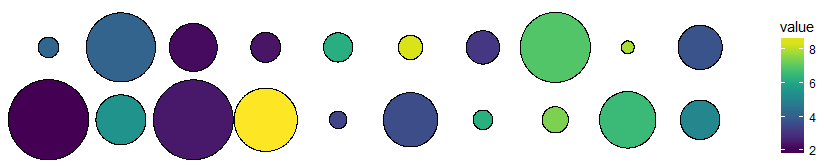
----     28 PARAMETER v  value

i1  4.237,    i2  4.163,    i3  2.183,    i4  2.351,    i5  6.302,    i6  8.478,    i7  3.077,    i8  6.992
i9  7.983,    i10 3.733,    i11 1.994,    i12 5.521,    i13 2.442,    i14 8.852,    i15 3.386,    i16 3.572
i17 6.346,    i18 7.504,    i19 6.654,    i20 5.174


----     28 PARAMETER r  radius

i1  1.273,    i2  4.295,    i3  2.977,    i4  1.855,    i5  1.815,    i6  1.508,    i7  2.074,    i8  4.353
i9  0.802,    i10 2.751,    i11 4.992,    i12 3.104,    i13 4.960,    i14 3.930,    i15 1.088,    i16 3.379
i17 1.218,    i18 1.625,    i19 3.510,    i20 2.459


----     28 PARAMETER a  area

i1   5.090,    i2  57.945,    i3  27.837,    i4  10.812,    i5  10.349,    i6   7.146,    i7  13.517,    i8  59.535
i9   2.021,    i10 23.775,    i11 78.274,    i12 30.275,    i13 77.291,    i14 48.525,    i15  3.720,    i16 35.864
i17  4.659,    i18  8.299,    i19 38.709,    i20 18.998


----     28 PARAMETER W                    =       15.000  
            PARAMETER H                    =       10.000  

The area was computed with the familiar formula: \(a_i = \pi r_i^2\). The mathematical model can look like:\[\bbox[lightcyan,10px,border:3px solid darkblue]{\begin{align}\max\>&\sum_i v_i \delta_i\\ & (x_i-x_j)^2 + (y_i-y_j)^2 \ge (r_i+r_j)^2 \delta_i \delta_j & \forall i\lt j \\ & r_i \le x_i \le W - r_i\\ & r_i \le y_i \le H - r_i\\ &\delta_i \in \{0,1\}\end{align}}\] Here the binary variable \(\delta_i\) indicates whether we select circle \(i\) for inclusion in the container. The variables \(x_i\) and \(y_i\) determine the location of the selected circles.

This turns out to be a small but difficult problem to solve. The packing problem is a difficult non-convex problem in its own right and we added a knapsack problem on top of it.

In [1] we found the following solutions:


SolverObjective
Local solver (BONMIN)58.57
Improved by global solver (LINDOGLOBAL)60.36

Combinatorial Benders Decomposition


In the comments of [1] a variant of Benders Decomposition called Combinatorial Benders Decomposition is suggested by Rob Pratt. Let's see if we can reproduce his results. I often find it useful to do such an exercise to fully understand and appreciate a proposed solution.

First, lets establish that the total number of solutions in terms of the binary knapsack variables \(\delta_i\) is: \(2^n\). For \(n=20\) we have: \[2^{20} = 1,048,576\] This is small for a MIP. In our case unfortunately we have this non-convex packing sub-problem to worry about.

One constraint that can be added is related to the area: the total area of the selected circles should be less than the total area of the container: \[\sum_i a_i \delta_i \le A\] where \(A=W \times H\). This constraint is not very useful to add to our MIQCP directly, but it will be used in the Benders approach. The number of  solutions for \(\delta_i\)  that are feasible w.r.t. the area constraint is only 60,145. The number of these solutions with a value larger than 60.3 is just 83.

To summarize:

SolutionsCount
Possible configurations for \(\delta_i\)1,048,576
Of which feasible w.r.t area constraint 60,145
Of which have a value better than 60.3 83

Now we have a number that is feasible to enumerate. We know the optimal objective value should be in this set of 83 problem that are better than 60.3. So a simple approach is just to enumerate solutions starting with the best.

We can give this scheme a more impressive name: Combinatorial Benders Decomposition[2]. The approach can be depicted as:


We add a cut in each iteration to the master. This cut \[\sum_{i\in S} (1-\delta_i)\ge 1\] where \(S = \{i|\delta_i=1\}\), will cut off exactly one solution. In theory it can cut off more solutions, but because of the order we generate proposals, just one solution is excluded each cycle.

The sub model is used only to see if the proposal is feasible w.r.t. to our rectangle. The first sub problem that is feasible gives us an optimal solution to the whole problem.  I implement the sub problem as a multistart NLP problem [3]. A slight rewrite of the sub problem gives a proper optimization problem:\[\begin{align} \max \>& \phi\\& (x_i-x_j)^2 + (y_i-y_j)^2 \ge \phi (r_i+r_j)^2&i\lt j\end{align}\] If the optimal value \(\phi^* \ge 1\) we are feasible w.r.t. to the original problem.

Of course, we could as well generate all possible configurations \(\delta_i\) that are feasible w.r.t. to the area constraint (there are 60,145 of them), order them by value (largest value first) and run through. Stop as soon as we find a feasible solution (i.e. where the packing NLP is feasible). No fancy name for this algorithm: "sorting" does not sound very sophisticated.

We can find a better solution with value 60.6134 using this scheme. Of course it is not easy. We need to solve 69 rather nasty non-convex NLPs to reach this solution.

Best Solution Found
Better than just solving the complete knapsack problem directly, but still not a panacea: this remains a small but surprisingly difficult problem to solve!

References


  1. Knapsack + packing: a difficult MIQCP, http://yetanothermathprogrammingconsultant.blogspot.com/2018/05/knapsack-packing-difficult-miqcp.html
  2. Codato G., Fischetti M. (2004) Combinatorial Benders’ Cuts. In: Bienstock D., Nemhauser G. (eds) Integer Programming and Combinatorial Optimization. IPCO 2004. Lecture Notes in Computer Science, vol 3064. Springer, Berlin, Heidelberg
  3. Multi-start Non-linear Programming: a poor man's global optimizer, http://yetanothermathprogrammingconsultant.blogspot.com/2018/05/multi-start-non-linear-programming-poor.html

Friday, May 25, 2018

DIY Presolve

In certain models, we can choose some level of "presolve" at the model level. Presolvers are part of LP/MIP solvers. Their main task is to inspect the model and look for opportunities to make it smaller. Some of this is done by simple operations such as: change a singleton constraint into a bound, remove variables that are not needed, etc [2,3].

Note that the meaning of "smaller" in this context is not totally obvious: some substitutions will decrease the number of decision variables and constraints, while increasing the number of non-zero coefficients in the LP matrix. Usually larger and sparser is better than smaller and denser (most LP and MIP solvers exploit sparsity), so I tend to focus on nonzero counts.

The question I am exploring here: how many reductions do we apply at the modeling level opposed to leave it to solver? If a solver is able to reduce the size by a large amount (loosely defined), I always feel I did not do a good job as a modeler. I just did not pay attention.

The model below demonstrates how we can apply different reduction levels to the model. The model becomes smaller, but at the expense of more complex modeling. What is the right level to choose? Of course there is no objective answer to this. Your "optimal level" may be different from mine.

Problem description


The problem is from [1]. Consider the board:


We need to fill the board with integers: \(x_{i,j} \in Z\). The following rules apply:

  1. Green cells must contain strictly positive values, \(x_{i,j}\ge 1\).
  2. Red cells must contain strictly negative values, \(x_{i,j}\le -1\).
  3. White and blue cells have a value of zero, \(x_{i,j}= 0\).
  4. The red and green cells form a symmetric pattern: if \(x_{i,j}\) is a green cell, \(x_{j,i}\) is a red cell, and the other way around.    
  5. Skew-symmetry or Anti-symmetry: we have the restriction \(x_{i,j} = -x_{j,i}\). Putting it differently: \(X^T = -X\).
  6. Row and column sums are equal to zero: \[ \begin{align}&\sum_i x_{i,j} =0 & \forall j\\& \sum_j x_{i,j} = 0 & \forall i\end{align}\]
There are multiple solutions. We may choose the solutions with the smallest sum of green values:\[\min \sum_{\mathit{Green}(i,j)} x_{i,j}\]

In the board above we have the following statistics:

Cell typeCount
Green cells57
Red cells57
Blue cells20
White cells266
Total400


Presolve level 0


A direct formulation for all \(x_{i,j}\) is: \[\begin{align}\min\> & z=\sum_{\mathit{Green}(i,j)}  x_{i,j}\\ &  x_{i,j}\ge 1  & \mathit{Green}(i,j)\\ &  x_{i,j} \le  -1  & \mathit{Red}(i,j)\\  &  x_{i,j} =0  & \mathit{WhiteBlue}(i,j)\\ & x_{i,j} = -x_{j,i} & \forall i,j\\ &\sum_i x_{i,j} =0 & \forall j\\&\sum_j x_{i,j} =0 & \forall i \\ & x_{i,j} \in Z\end{align}\]

This model, with all equations stated as explicit constraints, has the following sizes:

Model SizeCount
rows840
columns400
nonzero elements1980

The counts here exclude the objective function. Although the solver will automatically convert singleton equations into bounds, I never write these as explicit constraints. I prefer to specify singleton equations as bounds.

Presolve level 1


The first three constraints can be implemented as bounds: \[\ell_{i,j} = \begin{cases} 1 & \mathit{Green}(i,j)\\ -\infty & \mathit{Red}(i,j)\\  0 & \text{otherwise}\end{cases}\] and \[u_{i,j} = \begin{cases} \infty & \mathit{Green}(i,j)\\ -1& \mathit{Red}(i,j)\\ 0 & \text{otherwise}\end{cases}\] Now the model can read: \[\begin{align}\min \> & z=\sum_{\mathit{Green}(i,j)}  x_{i,j}\\ &   x_{i,j} = -x_{j,i} & \forall i\lt j\\ &\sum_i x_{i,j} =0 & \forall j\\&\sum_j x_{i,j} =0 & \forall i\\ & x_{i,j} \in [\ell_{i,j}, u_{i,j}] \\& x_{i,j} \in Z\end{align}\] I also reduced the number of skew-symmetry constraints \(x_{i,j}=-x_{j,i}\): we only need these for \(i\lt j\). This reduces the model size to:

Model SizeCount
rows230
columns400
nonzero elements1180

All singleton equations have been formulates as bounds. This model has a large number of variables fixed to zero (all variables corresponding to blue and white cells). The solver will presolve those variables away, but I prefer to do this myself.

Presolve level 2


The next level is to remove all \(x_{i,j}\) that are known to be zero from the model. \[\begin{align}\min \> & z= \sum_{\mathit{Green}(i,j)}  x_{i,j}\\ &   x_{i,j} = -x_{j,i} & \forall \mathit{Green}(i,j)\\ &\sum_{i|\mathit{GreenRed}(i,j)} x_{i,j} =0 & \forall j\\&\sum_{j|\mathit{GreenRed}(i,j)} x_{i,j} =0 & \forall i\\ & x_{i,j} \in [\ell_{i,j}, u_{i,j}] & \forall \mathit{GreenRed}(i,j)\\& x_{i,j} \in Z\end{align}\] The only cells we model here are the red and green ones. Our counts are:

Model SizeCount
rows97
columns114
nonzero elements342

This was my first actual implementation. However, we can go further, and use some more  reductions. Here the model starts to become less intuitive.

Presolve level 3


We can implicitly deal with the red cells: a red cell \(x_{i,j}\) has a corresponding green cell \(-x_{j,i}\). \[\begin{align}\min \> & z=\sum_{\mathit{Green}(i,j)}  x_{i,j}\\  &  \sum_{i|\mathit{Green}(i,j)}  x_{i,j} - \sum_{i|\mathit{Green}(j,i)}x_{j,i} =0 & \forall j\\&\sum_{j|\mathit{Green}(i,j)} x_{i,j} - \sum_{j|\mathit{Green}(j,i)} x_{j,i} =0 & \forall i\\ & x_{i,j} \ge 1 & \forall \mathit{Green}(i,j)\\& x_{i,j} \in Z\end{align}\] We only solve for the green cells here. The value of the red cells can be recovered afterwards.

Model SizeCount
rows40
columns57
nonzero elements228

The row and column sums now become more difficult to recognize. In addition we need to add some code to recalculate the value of the red cells after the solve.

Presolve level 4


Finally, we can also remove one of the summations because of symmetry. We end up with: \[\begin{align}\min \> & z=\sum_{\mathit{Green}(i,j)}  x_{i,j}\\  &  \sum_{i|\mathit{Green}(i,j)}  x_{i,j} - \sum_{i|\mathit{Green}(j,i)}x_{j,i} =0 & \forall j\\ & x_{i,j} \ge 1 & \forall \mathit{Green}(i,j)\\& x_{i,j} \in Z\end{align}\]
Model SizeCount
rows20
columns57
nonzero elements114

Again, the value of the red cells need to be calculated after the solve. This model is now very compact, but we moved away from the original problem statement. When reading this model, we would not immediately see the correspondence with the problem.

Does it make a difference?


No. The first model shows:

Presolved: 13 rows, 48 columns, 96 nonzeros
Variable types: 0 continuous, 48 integer (0 binary)

The last model gives:

Presolved: 13 rows, 48 columns, 96 nonzeros
Variable types: 0 continuous, 48 integer (0 binary)
So should we even worry? I still like to generate models that are somewhat small. For me this is not even a performance issue, but rather a question of paying attention. I see sometimes sloppy modeling causing an excessive number of variables, equations and nonzero elements. How far I take this DIY presolve effort is determined by readability and understandability: the limit is when the formulation becomes less obvious and when readability starts to suffer.

In any case, if the solver can presolve large parts of the model away, I want to be able to explain this. May be the model is largely triangular, or there are many singleton equations. Things may be more complex, and such an explanation is not always obvious to find.

Solution


The solutions looks like:


The minimum sum of the green cells is 87.


Update: fixed reference: use proper names of authors.

References


  1. Antisymmetric Table Puzzle where the rows/columns sum to zero. https://math.stackexchange.com/questions/2794165/antisymmetric-table-puzzle-where-the-rows-columns-sum-to-zero
  2. A.L. Brearley, G. Mitra, H.P. Williams, Analysis of mathematical programming problems prior to applying the simplex algorithm, Mathematical Programming, 8 (1975), pp. 54-83.
  3. E.D. Andersen, K.D. Andersen, Presolving in Linear Programming, Mathematical Programming, 71 (1995), pp. 221-245.

Wednesday, May 23, 2018

Excel Power Query CSV read somewhat slow

Reading a large CSV file into Excel's data model is somewhat slow compared to R: Excel/Power Query takes 100 seconds vs R only 25 seconds on the same CSV file (with 1.8 million records).

Reading CSV into Excel/Power Query data model
I used some VBA code for the timing. The only thing we do is to load data into the data model (i.e. there is no Power Pivot table to create).

R does this quite a bit faster:

Reading the same CSV into R
I expected this to be closer. I think this operation should be IO bound instead of CPU bound, something Microsoft should know how to do super fast.

Monday, May 21, 2018

Find the differences: RStudio local or server


Typically I run RStudio locally. For a project we are experimenting with RStudio Server, which allows you to run Rstudio itself on a server and use it from a web browser. The GUI looks virtually identical. The user experience is very similar (things like filenames are the main difference: the server is Linux based while I run Rstudio locally on Windows).

Sunday, May 20, 2018

Facility location model Q&A


Dear Erwin, 
I always follow and read your interesting posts. Thank you so much for your useful posts on your blogs. For the learning purposes, I was trying to code you MIQCP sample on your blog but not successful.  (http://yetanothermathprogrammingconsultant.blogspot.com.au/2018/01/solving-facility-location-problem-as.html). 
I have checked the code, Lp, and your post 10,000 times. Everything seems to be exactly like what you have addressed however not sure why Gams returns the error as 100 nonlinear lines. I see you are too busy and not work as GAMS support. But since it might be a coding problem with your post (or perhaps something is missed), It would be highly appreciated if you could do a favor and double check that. Much obliged.  

The attached GAMS model looks like:


set i /i1*i50/
set j /facility1,facility10/

parameter maxdist /40/;

set c /x,y/

Table dloc(i,c)
           x         y
i1         65        84
i2         8         72
i3         57        28
i4         70        79
i5         82        80
i6         87        95
i7         14        98
i8         28        6
i9         62        22
i10        22        80
i11        31        94
i12        87        74
i13        80        32
i14        92        48
i15        22        74
i16        0         42
i17        80        90
i18        100       56
i19        73        1
i20        82        84
i21        7         15
i22        3         19
i23        99        89
i24        56        94
i25        18        35
i26        8         30
i27        71        19
i28        10        66
i29        7         71
i30        13        66
i31        68        14
i32        95        43
i33        23        50
i34        95        43
i35        4         63
i36        51        13
i37        56        26
i38        41        56
i39        75        72
i40        41        68
i41        57        91
i42        16        63
i43        75        82
i44        44        94
i45        79        32
i46        72        5
i47        4         52
i48        16        20
i49        31        60
i50        92        63
;

scalar M /1000000/

variable
   floc(j,c)
   n

binary variables
  isopen(j)
  assign(i,j)

equations
   distance,assigndemand,closed,numfacilities,order;

distance(i,j)..          (sum(c,dloc(i,c)- floc(j,c)))**2 =l= Maxdist**2 + M*(1-assign(i,j));
assigndemand(i)..         Sum(j,assign(i,j)) =e= 1;
closed(i,j)..             assign(i,j) =l= isopen(j) ;
Numfacilities..           n =e= sum(j,isopen(j));
order(j+1)..              isopen(j) =g= isopen(j+1);

model location /all/

option limcol = 180;
option limrow =180;

solve location minimizing n using MIQCP;

display n.l,floc.l;


I think this GAMS model as written has a few problems that are interestingly enough to point out.

What is this about?


In [1] a simple facility location problem was discussed. It comprised of two models:

  1. Find the number of facilities \(n\) needed, so all demand locations are within MAXDIST kilometers from the closest facility.
  2. Given that we know \(n\), place these \(n\) facilities such that some total distance measure is minimized. 
The first model is presented as:


What is wrong with the GAMS model in the e-mail?


Quite a few things. Let me try to review them:

  1. The set \(j\) only has two elements. This is not sufficient. We should have more elements in \(j\) than the optimal value of \(n\).  The optimal value for this data set is \(n^* = 3\), so just having two elements in \(j\) will cause the model to be infeasible.
  2. The value for \(M\) needs to get much more attention. The value needs to be large enough that the distance equation becomes non-binding when \(\mathit{assign}_{i,j}=0\). A simple value would be \[M=\sum_c \left(\max_i \{ \mathit{dloc}_{i,c}\} -\min_i \{\mathit{dloc}_{i,c}\}\right)^2 \] This is the square of the length of the diagonal of the box containing all demand locations. For this data this leads to \(M=19409\). 
    We can assume facilities will be placed in the convex hull of the demand locations (sorry, I don't know how to prove that). That means we can use the maximum pairwise squared distance between demand locations \((i,i')\) as a good value for \(M\): \[M= \max_{i,i'} \sum_c \left(\mathit{dloc}_{i,c}-\mathit{dloc}_{i',c}\right)^2\] This sets \(M=14116\).
    With some effort better values can be derived by using individual values \(M_{i,j}\) instead of one \(M\). Big-M values with some computation and just having assigned some large value, are always a point of attention.
    Using just very big values for big-\(M\) constants, is something I see very often. This can lead to all kind of problems when solving the MIP problem. 
  3. The expression (sum(c,dloc(i,c)- floc(j,c)))**2 takes the square of the sum. This is not the same as a sum of squares:\[\sum_i x_i^2 \ne \left(\sum_i x_i\right)^2\] This expression is just malformed.
  4. In GAMS x**y is a general non-linear function, and x**2 is not recognized as quadratic function (GAMS could be much smarter here). This will make the model an MINLP model and not a MIQCP. This will lead to the somewhat cryptic error:

      --- Executing SBB: elapsed 0:00:00.140
      Could not load data
      Detected 100 general nonlinear rows in model


    Of course you can solve it with an MINLP solver. (Confusingly SBB is an MINLP solver).  Of course it is better to use the sqr(x) function to help GAMS. The left-hand side of the distance constraint should be written as: sum(c,sqr(dloc(i,c)- floc(j,c))).
    Side note: if we would try to solve the original expression (sum(c,dloc(i,c)- floc(j,c)))**2 as a MINLP model, we would still be in a heap of problems. The function x**y assumes \(x\ge 0\). This is obviously not the case here. We would see a ton of domain errors. 
  5. For an optimal solution, you will need to add: option optcr=0; GAMS has a default relative gap tolerance of 10%. With this options we set this tolerance to zero.
Modeling is not that easy! We need to pay attention to lots of details to get models working correctly.

Wednesday, May 16, 2018

Coming to Excel: custom R plots

Interesting. Excel's charts are looking a bit dated compared to what we can do with ggplot, plot.ly or Tableau. This will make a good step in the right direction.


Sankey Chart in Excel


References

  1. Custom R charts coming to Excel, http://blog.revolutionanalytics.com/2018/05/powerbi-custom-visuals-in-excel.html
  2. Azure Machine Learning, JavaScript Custom Functions, and Power BI Custom Visuals Further Expand Developers Capabilities with Excel, https://dev.office.com/blogs/azure-machine-learning-javascript-custom-functions-and-power-bi-custom-visuals-further-expand-developers-capabilities-with-excel
  3. Excel announces new data visualization capabilities with Power BI custom visuals,  https://powerbi.microsoft.com/en-us/blog/excel-announces-new-data-visualization-capabilities-with-power-bi-custom-visuals/

Indicator constraints

In [1] a question is posed about how to implement the implication:\[ x+y\le 5 \Rightarrow \delta = 1\] Here \(\delta \in \{0,1\}\) is a binary variable. Indicator constraints are of the form:\[ \delta = 0 \Rightarrow \text{constraint}\] or \[ \delta = 1 \Rightarrow \text{constraint}\] The binary variable \(\delta\) is sometimes called an indicator variable.

From propositional logic we have: \[\begin{align} & A \Rightarrow B \\ & \Leftrightarrow \\  & \neg B \Rightarrow \neg A\end{align}\] This is called transposition [2].

From this, we can formulate:\[\delta = 0 \Rightarrow x+y\gt 5\] If \(x\) or \(y\) is a continuous variable we can choose to write \[\delta = 0 \Rightarrow x+y\ge 5.001\] or just \[\delta = 0 \Rightarrow x+y\ge 5\] In the latter case we keep things ambiguous for \( x+y=5\) which is in practice often a good choice.

If  \(x\) and \(y\) are integers, we can do: \[\delta = 0 \Rightarrow x+y\ge 6\]

This trick is quite useful to know when dealing with indicator constraints.

References


Overdoing a plot


Lots of things are going on here. This is a visualization of a packing problem: place 50 circles in a square that is as small as possible, Things are solved by 50 solves by SNOPT with a random starting point (i,e, a multi-start approach).

  1. On the left we have the best packing so far. The small light-blue area indicates how much we improved on the first solve.
  2. The second plot shows the objective function value of each solve. The red line is the best objective so far.
  3. The density plot shows the probability of a better solution out there. Just using a normal distribution. The blue area is the probability. The blue area is the tail area corresponding to the red line in the second picture.
  4. The last plot shows these probabilities in a different format. The trend is downhill, but not uniformly so.
I went a bit overboard with my ggplot scripts....

Sunday, May 13, 2018

100% accurate

Hi Erwin,
I have few doubts 
i found you in search of regularization topic 
I have done multiple regression and i observed there is over fitting in my predicted results
My  CEO need 100% accurate predicted model but i don't know how to do regularization for multiple linear regression using excel. Could you please let me know how to do it in a step wise manner or share me any article related to it if you have 

Thank You

I am glad I am not working for that CEO.

Multi-start Non-linear Programming: a poor man's global optimizer

If a nonlinear optimization problem is non-convex, a local solver typically will find a locally optimal solution. If the model is not too large, we may find a globally optimal solution by invoking a global solver such as Baron.


Global optimization of packing problem by multi-start NLP


In [1] the following non-convex model is used to pack \(n=50\) circles in a square that is as small as possible:

\[\begin{align} \min_{x,y,S}\>&S\\ &(x_i - x_j)^2 +(y_i - y_j)^2 \ge (r_i+r_j)^2 &\forall i \lt j\\ & r_i \le x_i \le S- r_i \\ & r_i \le y_i \le S - r_i\end{align}\]

This is a difficult model for global solvers. In the animation above we solve \(N=50\) problems with a different random starting point using SNOPT (a local NLP solver). The random starting points we generate are not feasible. SNOPT seems to have no problems in finding a feasible and locally optimal configuration. The results look quite good. Sometimes a really lo-tech approach is quite appropriate.

Speeding up the solve loop in GAMS


Here we do some experiments with a loop of \(N=50\) tries, each with \(n=50\) circles to be packed. 
  1. A simple loop statement is the most obvious approach. On my machine this takes 73 seconds.
  2. Speed up the loop by using a solver DLL (instead of a .EXE), and reducing output in the listing file (m.solprint=2) . The elapsed time is now 40 seconds.
  3. Run all 50 problems in parallel using solvelink.async (we kept m.solprint=2). The total time reduces to 16 seconds. 
  4. Add extra logic to run up to 4 jobs at the time (my laptop has 4 real cores). This does not help. It increases the run time to 40 seconds. The effort to start a new job once a running job is finished adds some idle time. Looks like it is better to keep things saturated and launch all our jobs. This assumes we have enough memory to keep all jobs in RAM. 
  5. Scenario solver. This multi-start algorithm can be considered as solving \(N\) independent scenarios. It would be a good candidate for the GAMS scenario solver [2]. The scenario solver allows independent scenarios to solve very efficiently by updating the problem directly in memory. Unfortunately, this tool is not flexible enough to be able to handle a multi-start approach (we cannot initialize the levels before each solve).

Stopping rule


In this experiment we simply ran \(N=50\) jobs. A more sophisticated approach would be to use a probabilistic argument for stopping the search [3]: stop when the probability of finding a better solution becomes small.

Looking at the objectives in the plot above, it looks they may be normally distributed,


Apart from the outlier (the last solve), this indeed looks to be the case. The idea is to track the probability we can find an objective that is better than the current best one:

The blue area in the density plot is the probability we can improve the objective


Multi-start and global solvers


The global solve Baron actually runs a few multi-start solves inside to try to improve the initial solution:

  Starting multi-start local search
  Done with local search

In this case it did not improve anything. Besides this we can run our own multi-start algorithm, Baron automatically picks up a good solution from the initial values:

  Starting solution is feasible with a value of    0.269880944180E-001 


A related problem


A similar problem is the "hostile brothers problem". Given a plot of land (here \([0,1]\times [0,1]\)), place \(n\) points such that the minimum distance is maximized. The model can look like:

\[\begin{align} \max_{x,y,d^2}\>&d^2\\ &d^2 \le (x_i - x_j)^2 +(y_i - y_j)^2 &\forall i \lt j\\ & x_i, y_i \in [0,1]\end{align}\]

Again, good solutions can be found using a simple multi-start strategy,

Hostile Brothers Problem solved with a multi-start algorithm

In this case it is very easy to generate a feasible starting point:\[\begin{align}&x_i \sim U(0,1)\\&y_i \sim U(0,1)\\& d^2 := \max_{i\lt j} \left\{ (x_i - x_j)^2 +(y_i - y_j)^2 \right\} \end{align}\]

References


  1. Knapsack + packing: a difficult MIQCP, http://yetanothermathprogrammingconsultant.blogspot.com/2018/05/knapsack-packing-difficult-miqcp.html
  2. Gather-Update-Solve-Scatter (GUSS), https://www.gams.com/latest/docs/S_GUSS.html
  3. C.G.E. Boender and A.H.G. Rinnooy Kan. Bayesian stopping rules for multistart global optimization methods. Mathematical Programming, 37:59–80, 1987
  4. Stopping criteria for meta-heuristics, http://yetanothermathprogrammingconsultant.blogspot.com/2015/01/stopping-criteria-for-meta-heuristics.html

Wednesday, May 9, 2018

Knapsack + packing: a difficult MIQCP


Packing Circles in a Rectangle


The problem of placing the maximum number of circles (or spheres) with radius \(r\) in a container (e.g. rectangle or box) such that there is no overlap is a well-known packing problem. Another version is: minimize the size of the container, such that it can contain \(n\) spheres. In [1] some nice pictures are produced for different type of containers:

Smallest containers with 100 balls. Picture from [1]


Smallest container problem


The problem of finding the smallest enclosing box to fit \(n\) circles (spheres) with radius \(r_i\), can be stated as a quadratic problem: \[\begin{align} \min\>&S\\ &(x_i - x_j)^2 +(y_i - y_j)^2 \ge (r_i+r_j)^2 &\forall i \lt j\\ & r_i \le x_i \le S- r_i \\ & r_i \le y_i \le S - r_i\end{align}\] For the 3D case, just extend this model with \(z_i\).

This looks like a simple model, but it is not. The constraints are non-convex, so solvers like Cplex and Gurobi are out the window.  Global solvers like Baron, Couenne and Antigone have a very tough time on this model. Even for \(n=10\) points they have troubles finding a proven optimal solution.

A simple heuristic that works well, is to solve this with a local solver (I used SNOPT here) using a multi-start approach. To make things easy, I just ran \(N=25\) copies of the problem simultaneously, each with a different random starting point.

Notes:

  • My solutions are marginally worse than reported in [3]. One reason is that SNOPT is using tighter tolerances than [3]: their solutions are declared infeasible by SNOPT. The circles in [3] just slightly overlap.
  • I simply used random starting point (to be precise: random locations in a larger box than I would expect the final solution to be). It may be interesting to see if we can do better, such as trying to generate a feasible starting point. Alternatively, we could start with circle organized in a grid and then jitter them a bit by a random perturbation.
  • I  ran all 25 solves in parallel. My laptop has 4 real cores, so it may be slightly better to run 4 problems in parallel. I doubt this will make much difference. 
  • Circles and spheres are somewhat easy. If the items are boxes, we need to worry about possible rotations. 
  • In [2] a slightly different formulation is used. Instead of having \((x_i - x_j)^2 +(y_i - y_j)^2 \ge (r_i+r_j)^2\) for each \(i\lt j\), we can do \[\min_{i \lt j} \left[ (x_i - x_j)^2 +(y_i - y_j)^2 -(r_i+r_j)^2\right] \ge  0\] Instead [2] proposes:  \[\sum_{i\lt j} \left[ \max\{0,(r_i+r_j)^2- (x_i - x_j)^2 -(y_i - y_j)^2 \}   \right]^2 = 0 \] The outer squares are used to alleviate that \(\max\{0,x\}\) is non-differentiable: the function \(\left( \max\{0,x\}\right)^2 \) is differentiable.

A problem with \(n=50\) circles with radius \(r_i=1\) can be packed in a square of size \(S=14.021\).


A second problem with \(n=50\) and \(r_i \sim U(0,2)\) (i.e. uniform between 0 and 2) needs a slightly larger square with \(S=14.598\). Now we get the more psychedelic plot:


Knapsack problem


We can make this problem a lot more difficult. Suppose we have a collection of circles with a value \(v_i\) and a radius \(r_i\). Given a rectangular container of size \(W \times H\) try to design a payload with maximum value. Our random data looks like:


----     19 PARAMETER v  value

i1  4.237,    i2  4.163,    i3  2.183,    i4  2.351,    i5  6.302,    i6  8.478,    i7  3.077,    i8  6.992
i9  7.983,    i10 3.733,    i11 1.994,    i12 5.521,    i13 2.442,    i14 8.852,    i15 3.386,    i16 3.572
i17 6.346,    i18 7.504,    i19 6.654,    i20 5.174


----     19 PARAMETER r  radius

i1  1.273,    i2  4.295,    i3  2.977,    i4  1.855,    i5  1.815,    i6  1.508,    i7  2.074,    i8  4.353
i9  0.802,    i10 2.751,    i11 4.992,    i12 3.104,    i13 4.960,    i14 3.930,    i15 1.088,    i16 3.379
i17 1.218,    i18 1.625,    i19 3.510,    i20 2.459


----     19 PARAMETER d  diameter

i1  2.546,    i2  8.589,    i3  5.953,    i4  3.710,    i5  3.630,    i6  3.016,    i7  4.148,    i8  8.706
i9  1.604,    i10 5.502,    i11 9.983,    i12 6.209,    i13 9.920,    i14 7.860,    i15 2.176,    i16 6.757
i17 2.436,    i18 3.251,    i19 7.020,    i20 4.918

We want to place as many high-valued and small circles in our rectangle:

Color coded items we can place in our rectangular knapsack
The rectangular container for this problem has \(W=15, H=10\).

The model to select the most valuable payload can be formulated as:\[\begin{align}\max\>&\sum_i v_i \delta_i\\ & (x_i-x_j)^2 + (y_i-y_j)^2 \ge (r_i+r_j)^2 \delta_i \delta_j & \forall i\lt j\\ & r_i \le x_i \le W - r_i\\ & r_i \le y_i \le H - r_i\\ &\delta_i \in \{0,1\}\end{align}\] Here the binary variable \(\delta_i\) indicates whether we select circle \(i\) for inclusion in the container.

Instead of \((x_i-x_j)^2 + (y_i-y_j)^2 \ge (r_i+r_j)^2 \delta_i \delta_j\), we can use a big-M constraint: \[(x_i-x_j)^2 + (y_i-y_j)^2 \ge (r_i+r_j)^2 - (1-\delta_i) M_{i,j} - (1-\delta_j) M_{i,j} \] with \(M_{i,j}=(r_i+r_j)^2\). Rewriting this a bit leads to: \[(x_i-x_j)^2 + (y_i-y_j)^2 \ge M_{i,j} (\delta_i + \delta_i - 1)\]

This is a MIQCP (Mixed Integer Quadratically Constrained Problem). Again, commercial solvers like Cplex and Gurobi don't help us here. We can try to solve this with a local MINLP solver or be ambitious and use a global solver. Even though we can not prove optimality, we can try to get a good solution with a local solver and then improve the solution with a global solver.

The local solvers (SBB, DICOPT, BONMIN) seem to like formulation \( (x_i-x_j)^2 + (y_i-y_j)^2 \ge (r_i+r_j)^2 \delta_i \delta_j \) better. BONMIN finds a solution of 58.57. LINDOGlobal is able to improve this to 60.36. The solution looks like:


----     92 VARIABLE delta.L  select

i1  1.000,    i4  1.000,    i5  1.000,    i6  1.000,    i7  1.000,    i9  1.000,    i12 1.000,    i15 1.000
i17 1.000,    i18 1.000,    i20 1.000


----     92 VARIABLE x.L  

i1   1.273,    i2   7.726,    i3   3.777,    i4   7.983,    i5   4.313,    i6  13.492,    i7   2.074,    i8  10.647
i9   3.980,    i10  5.454,    i11  5.769,    i12  7.721,    i13  7.856,    i14 11.070,    i15 13.912,    i16 10.971
i17 11.610,    i18  1.625,    i19  4.373,    i20 12.541


----     92 VARIABLE y.L  

i1  1.273,    i2  5.705,    i3  4.005,    i4  1.855,    i5  1.815,    i6  6.350,    i7  7.926,    i8  4.991
i9  5.771,    i10 4.268,    i11 4.992,    i12 6.896,    i13 5.040,    i14 5.713,    i15 8.912,    i16 5.312
i17 8.782,    i18 4.253,    i19 5.705,    i20 2.459

Plotting leads to:

Circles selected for 15 x 10 container. Unselected circles are plotted with transparent color.

Interestingly we don't select the most valuable circle i14. Note that this is not a proven globally optimal solution. To do a sanity check, I fixed \(\delta_{i14}=1\) and retried. Indeed I was not able to beat the best total value of  60.36.

References


  1. Ernesto G. Birgin, Applications of nonlinear programming to packing problems, in Applications + Practical Conceptualization + Mathematics = fruitful Innovation, Proceedings of the Forum of Mathematics for Industry 2014, R. S. Anderssen, P. Broadbridge, Y. Fukumoto, K. Kajiwara, T. Takagi, E. Verbitskiy, and M. Wakayama (Eds.), Springer Series Mathematics for Industry 11, pp. 31-39, 2016
  2. E. G. Birgin and F. N. C. Sobral, "Minimizing the object dimensions in circle and sphere packing problems", Computers & Operations Research 35, pp. 2357-2375, 2008.
  3. Packing Circles and Spheres using nonlinear programming, https://www.ime.usp.br/~egbirgin/packing/packing_by_nlp
  4. Mhand Hifi and Rym M'Hallah, “A Literature Review on Circle and Sphere Packing Problems: Models and Methodologies,” Advances in Operations Research, vol. 2009, Article ID 150624, 22 pages, 2009. https://doi.org/10.1155/2009/150624.