Friday, April 29, 2016

Excel: Simplex vs Evolutionary Engine (Simplex wins)

In this post a simple MIP problem is posted. Basically the problem can be stated as:

\[\boxed{\begin{align} \max & \sum_i Score_i \, x_i \\ & \sum_i x_i = 6 \\ & \sum_i Salary_i \, x_i \le 50000 \\ & x_i \in \{0,1\} \end{align}}\]

We have a database of 153 players, and we want to compose the best team of 6 players with a total salary cap of $50k. This can actually be done in Excel quite easily. With some random data I get the following results using the Simplex LP based MIP solver:

image

The name “Simplex LP” is somewhat misleading, as we solve here a MIP.

Some comments in the post are really surprising to me:

  • the number of combinations of 6 golfers from a pool of 153 is 16,133,132,940 Note that yes, that is over 16 billion combinations. Even if Solver can do it, it will probably crash Excel”. A MIP solver (or the Evolutionary Solver) will not evaluate all possible solutions! (That would be impossible in almost all cases). There is no reason to believe Excel will crash on this problem (quite the opposite: it solves quite quickly). I see this argument more often; apparently there are lots of people around who think complete enumeration is the best we can do.
  • Excel mentions “use Evolutionary engine for non-smooth problems” so one answer suggested to use the Evolutionary solver. Actually I understand why someone may think this is a wise decision: the hint can be interpreted as advice to use the Evolutionary algorithm for any discrete problem. Looking at the results below this is not such a good idea: the Evolutionary engine takes much more time and delivers a significantly sub-optimal solution. A summary comparison of the results is:

    image
  • The built-in version of Solver reports, ‘This problem is too large for Solver to handle.’ [..] an alternative is the free OpenSolver add-in (see opensolver.org)“ I have no idea why this user sees this message. I had no size problems using the sizes as indicated by the poster. This problem has 153 binary variables and I believe the limit is 200 variables.

Below is the result from a run with the same data using the Evolutionary solver:

image

Conclusion

My advice: always try a MIP model first. The model building process forces you to understand the problem better and a MIP solver can give proven optimal solutions (or a guaranteed quality when we allow a gap between best possible and best found solutions). If the performance is not satisfactory then consider using a meta-heuristic. (The MIP model an also be used then to debug the implement the meta-heuristic and compare the quality of the objective function values).

Wednesday, April 27, 2016

The end of (numeric) error

John Gustafson suggest to use a new data type called ‘unums’. They form a superset of the floating point numbers. "Unums are to floats what floats are to integers"

image

Sunday, April 24, 2016

Aircraft Landings

12027307554_cc95bbef64_z
Source.

In (1) and (2) an interesting problem is described: the aircraft landing problem. We have an airport with m runways, where we want to schedule aircrafts to land. Each aircraft has a target landing time and some allowed time window (it can land a bit earlier or somewhat later; typically the window is not symmetric around the target landing time). There is a required time between two landings (separation time) depending on the type of aircraft and the assigned runway. If two planes are scheduled on the same runway the separation time is longer than if they land on different runways.

The MIP model shown in (2) is as follows:

image


image

image

As usual I have some comments on the equations. Below I discuss each equations in turn (the numbers correspond to the equation number).

  1. The objective shows we have different costs for landing before or after the target landing time.
  2. This equation is just really a set of bounds that form the time-window. Usually I write these explicitly as bounds instead of constraints, even if presolvers will typically do this for you. When I specify them as bounds, I just want to convey in the model I know these restrictions are just bounds and paid attention.
  3. This constraint looks a bit unfamiliar, but actually is just a variable splitting constraint. Only one of \(a_i\), \(b_i\) will be nonzero due to the objective (if both are nonzero the LP solution of the current relaxation is not optimal).
  4. This constraint puts some limits on \(a_i\), but does not look like we need it. The first part: \(a_i \ge T_i-x_i\) follows from (3) while the bound \(a_i\le T_i-E_i\) follows from (2).
  5. This is similar and also looks redundant to me.
  6. This is a main constraint in the model. It says: if aircraft \(j\) is after \(i\) then there should be 1 or \(s_{i,j}\) minutes in between, depending on whether they land at the same runway. This equation gives rise to the thought we can make use of symmetry in the variables \(\delta_{i,j}\) (landing on same runway) and \(y_{i,j}\) (ordering). We know that \(\delta_{j,i} = \delta_{i,j}\) and that \(y_{j,i} = 1-y_{i,j}\). So we can save on these variables by exploiting that. Let’s say that we only have \(\delta_{i,j}\) and \(y_{i,j}\) for \(i<j\) (i.e. both are strictly upper triangular matrices) then we need to split constraint (6) into two parts:
    \[\begin{align} x_j-x_i  & \ge s_{i,j} \delta_{i,j} + (1 – \delta_{i,j}) – M(1-y_{i,j}) \>\> & \forall i<j \\
                         x_j-x_i  & \ge s_{i,j} \delta_{j,i} + (1 – \delta_{j,i}) – M y_{j,i} \>\> & \forall i>j \end{align}\]
    I am not sure if presolvers are so smart they can do this also. Even if they did, I would prefer to add this logic myself to show I have thought about this. We could do the same thing for \(s_{i,j}\) as the data seems to indicate \(s_{i,j}\) is symmetric. Saving on binary variables is more important that saving a few bytes on data, so we skip that. In addition, in practice \(s_{i,j}\) may not be symmetric (consider a Cessna before or after an A380).
    Of course we need to use a good value for \(M\) that is as small as possible. Probably we should use \(M_{i,j}\) instead (i.e. use several constants). Finally we note that if for a combination \(i,j\) the time windows are far away from each other we can even drop this equation altogether. I ignore this for now because the data sets I am looking at now do not have such combinations. 
  7. We can drop this constraint if we only consider \(y_{i,j}\) for \(i<j\). Of course we need to be careful when we use \(y_{i,j}\) in the model (see the discussion of the previous constraint).
  8. This constraint can be considered as a linearization of \(\delta_{i,j}=\max_r \gamma_{i,r}\gamma_{j,r}\). This is a multiplication of two binary variables. We can get rid of the max and linearize by
      \[ \delta_{i,j} \ge \gamma_{i,r}+\gamma_{j,r}-1\>\> \forall r, i\ne j \]
    Note that we let \(\delta_{i,j}\) float when aircraft \(i\) and \(j\) do not share a runway. The objective will drive it to zero when needed. Forcing \(\delta_{i,j}=0\) in that case is not so easy: we would need some intermediate variables for that.
    When we exploit symmetry we can reduce the number of constraints for equation (8). In our case it would become
    \[\delta_{i,j}\ge \gamma_{i,r} + \gamma_{j,r}-1 \>\> \forall r, i<j\] 
  9. Each aircraft has to land on exactly one runway.
  10. This equation can be deleted when we exploit symmetry ourselves. Note that the given domain: \(i,j=1,..,n, i\ne j\) for this equation seems a bit generous. I guess they mean \(i<j\).
  11. Here I would note that I would restrict the domains of \(\delta_{i,j}\) and \(y_{i,j}\) to \(i<j\). 
  12. When using a variable splitting technique I usually do not create two variables with different names (like \(a_i\) and \(b_i\)) but would rather create a single variable \(d_{i,k}\) (‘d’ for deviation from target landing time), where \(k=\{\text{early},\text{late}\}\). This is largely a matter of taste.

In summary, here is my version of the model:

image

The performance of the new formulation looks good at least on one small data set using 2 runways:

image

Some of the larger problems (n=44,n=50) are actually even easier to solve.

I am not sure how to depict the solution. Here is an attempt:

image

The dots indicate when a landing is scheduled and on which runway.

Conclusion

As usual: there is always a lot to think about, even for a small model like this.

References

(1) J. E. BEASLEY e.a., “Scheduling Aircraft Landings— The Static Case”, Transportation Science,Vol. 34, No. 2, May 2000

(2) Amir Salehipour, “Solving Large Aircraft Landing Problems on Multiple Runways by Applying a Constraint Programming Approach”, Report, The University of Newcastle, Australia, 2016

Friday, April 22, 2016

Dump solution data into a MySQL database II

This is a follow-up on this post. For large datasets using individual inserts is not as efficient as applying bulk operations. In MySQL bulk inserts can be done with the LOAD DATA LOCAL INFILE command. This statement takes a local (i.e. at the client) text file, copies it to the server and then does a bulk insert of the whole thing. This approach is built in the tool gdx2mysql. If a symbol has more than N records (N=500 by default), then we write a text file and call LOAD DATA LOCAL INFILE. If a symbol has fewer records then we just a standard prepared insert statement. A verbose log will show what happens.

set i /i1*i100/;
alias
(i,j,k);
parameter
a(i,j,k);
a(i,j,k) = uniform(0,100);
execute_unload "test"
,i,a;
execute "gdx2mysql -i test.gdx -s tmp -u test -p test -v";

In the above test model we generate a set with 100 elements and a parameter with 1003=1,000,000 elements. The verbose log looks like

--- Job Untitled_1.gms Start 04/22/16 04:01:39 24.6.1 r55820 WEX-WEI x86 64bit/MS Windows
GAMS 24.6.1   Copyright (C) 1987-2016 GAMS Development. All rights reserved
Licensee: Erwin Kalvelagen                               G150803/0001CV-GEN
          Amsterdam Optimization Modeling Group                     DC10455
--- Starting compilation
--- Untitled_1.gms(6) 3 Mb
--- Starting execution: elapsed 0:00:00.007
--- Untitled_1.gms(5) 36 Mb
--- GDX File C:\Users\Erwin\Documents\Embarcadero\Studio\Projects\gdx2mysql\Win32\Debug\test.gdx
--- Untitled_1.gms(6) 36 Mb
GDX2MySQL v 0.1
Copyright (c) 2015-2016 Amsterdam Optimization Modeling Group LLC

   GDX Library      24.6.1 r55820 Released Jan 18, 2016 VS8 x86 32bit/MS Windows
   GDX:Input file: test.gdx
   GDX:Symbols: 2
   GDX:Uels: 100
   GDX:Loading Uels
   SQL:Selected driver: MySQL ODBC 5.3 ANSI Driver
   SQL:Connection string: Driver={MySQL ODBC 5.3 ANSI Driver};Server=localhost;User=xxx;Password=xxx
      set autocommit=0
      select @@version_comment
   SQL:RDBMS: MySQL Community Server (GPL)
      select @@version
   SQL:RDBMS version: 5.6.26-log
      select count(*) from information_schema.schemata where schema_name = 'tmp'
   -----------------------
   i (100 records)
      drop table if exists `tmp`.`i`
      create table `tmp`.`i`(`i` varchar(4))
      insert into `tmp`.`i` values (?)
      sqlexecute(100 times)
      commit
      Time : 0.6
   a (1000000 records)
      drop table if exists `tmp`.`a`
      create table `tmp`.`a`(`i` varchar(4),`j` varchar(4),`k` varchar(4),`value` double)
      temp file: [C:\Users\Erwin\AppData\Local\Temp\tmpA046.tmp]
      writing C:\Users\Erwin\AppData\Local\Temp\tmpA046.tmp
      load data local infile 'C:\\Users\\Erwin\\AppData\\Local\\Temp\\tmpA046.tmp' into table `tmp`.`a`
      rows affected: 1000000
      commit
      Time : 39.6
      deleting [C:\Users\Erwin\AppData\Local\Temp\tmpA046.tmp]

*** Status: Normal completion
--- Job Untitled_1.gms Stop 04/22/16 04:02:20 elapsed 0:00:41.353

The smaller set i is imported using normal inserts, while the larger parameter a is imported through an intermediate text file. This is much more efficient than using the standard inserts. There is a gdx2mysql option to force larger symbols to use standard inserts, so we can compare timings:

a (1000000 records)
   drop table if exists `tmp`.`a`
   create table `tmp`.`a`(`i` varchar(4),`j` varchar(4),`k` varchar(4),`value` double)
   insert into `tmp`.`a` values (?,?,?,?)
   sqlexecute(1000000 times)
   commit 100 times
   Time : 257.5

So we are about 6.5 times as fast. (We can expect even larger differences in other cases).

A final way to make imports faster is to use ISAM (or rather MyISAM) tables. ISAM is an older storage format (MySQL nowadays uses the InnoDB storage engine by default). However ISAM is still faster for our simple (but large) tables, as can be seen when running with the –isam flag:

i (100 records)
   drop table if exists `tmp`.`i`
   create table `tmp`.`i`(`i` varchar(4)) engine=myisam
   insert into `tmp`.`i` values (?)
   sqlexecute(100 times)
   commit
   Time : 0.3
a (1000000 records)
   drop table if exists `tmp`.`a`
   create table `tmp`.`a`(`i` varchar(4),`j` varchar(4),`k` varchar(4),`value` double) engine=myisam
   temp file: [C:\Users\Erwin\AppData\Local\Temp\tmpBF31.tmp]
   writing C:\Users\Erwin\AppData\Local\Temp\tmpBF31.tmp
   load data local infile 'C:\\Users\\Erwin\\AppData\\Local\\Temp\\tmpBF31.tmp' into table `tmp`.`a`
   rows affected: 1000000
   commit
   Time : 9.9

This again makes a substantial difference in getting data into MySQL.

Finally a test using the a model with many symbols: indus89. It is noted that Cplex solves the LP model in less than a second and we need 29 seconds to store everything. Of course in practical situations we don’t store all symbols of a model (i.e. all sets, parameters, variables, equations - both input and output and intermediate results) but only solution information that is of interest. Here we use the default settings (i.e. non-verbose output).

--- Job indus89.gms Start 04/23/16 16:28:32 24.6.1 r55820 WEX-WEI x86 64bit/MS Windows
GAMS 24.6.1   Copyright (C) 1987-2016 GAMS Development. All rights reserved
Licensee: Erwin Kalvelagen                               G150803/0001CV-GEN
          Amsterdam Optimization Modeling Group                     DC10455
--- Starting compilation
--- indus89.gms(3624) 4 Mb
--- Starting execution: elapsed 0:00:00.067
--- indus89.gms(3618) 6 Mb
--- Generating LP model wsisn
--- indus89.gms(3621) 9 Mb
---   2,726 rows  6,570 columns  39,489 non-zeroes
--- Executing CPLEX: elapsed 0:00:00.459

IBM ILOG CPLEX   24.6.1 r55820 Released Jan 18, 2016 WEI x86 64bit/MS Windows
--- GAMS/Cplex licensed for continuous and discrete problems.
Cplex 12.6.3.0

Reading data...
Starting Cplex...
Space for names approximately 0.28 Mb
Use option 'names no' to turn use of names off
Tried aggregator 1 time.
LP Presolve eliminated 280 rows and 805 columns.
Aggregator did 652 substitutions.
Reduced LP has 1794 rows, 5113 columns, and 33006 nonzeros.
Presolve time = 0.09 sec. (6.67 ticks)
Initializing dual steep norms . . .

Iteration log . . .
Iteration:     1   Scaled dual infeas =       2955667.467575
Iteration:   145   Scaled dual infeas =            67.402987
Iteration:   320   Scaled dual infeas =            40.456945
Iteration:   456   Scaled dual infeas =             0.000000
Iteration:   457   Dual objective     =        693736.223395
Iteration:   566   Dual objective     =        357373.814662
Iteration:   698   Dual objective     =        323632.243202
Iteration:   841   Dual objective     =        287702.310223
Iteration:  1032   Dual objective     =        214777.339973
Iteration:  1186   Dual objective     =        197801.054391
Iteration:  1321   Dual objective     =        192342.788491
Iteration:  1493   Dual objective     =        165767.510563
Iteration:  1616   Dual objective     =        158191.208028
Iteration:  1778   Dual objective     =        145496.672263
Iteration:  1877   Dual objective     =        143045.603206
Iteration:  1989   Dual objective     =        139486.873101
Iteration:  2083   Dual objective     =        136581.639370
Iteration:  2207   Dual objective     =        133666.833792
Iteration:  2343   Dual objective     =        130050.280793
Iteration:  2466   Dual objective     =        127415.162363
Iteration:  2617   Dual objective     =        123160.882361
Iteration:  2725   Dual objective     =        121804.057461
Iteration:  2830   Dual objective     =        120796.202924
Iteration:  2954   Dual objective     =        118752.921229
Iteration:  3054   Dual objective     =        117126.856176
Iteration:  3148   Dual objective     =        116392.467557
Iteration:  3259   Dual objective     =        115780.645362
Iteration:  3351   Dual objective     =        115477.692660
Iteration:  3455   Dual objective     =        115194.050278
Iteration:  3543   Dual objective     =        114874.122256
Removing shift (1).
LP status(1): optimal
Cplex Time: 0.78sec (det. 245.24 ticks)

Optimal solution found.
Objective :      114873.655552

--- Restarting execution
--- indus89.gms(3621) 4 Mb
--- Reading solution for model wsisn
--- indus89.gms(3621) 4 Mb
--- Executing after solve: elapsed 0:00:02.716
--- indus89.gms(3623) 5 Mb
--- GDX File C:\Users\Erwin\Documents\Embarcadero\Studio\Projects\gdx2mysql\Win32\Debug\test.gdx
--- indus89.gms(3624) 5 Mb
GDX2MySQL v 0.1
Copyright (c) 2015-2016 Amsterdam Optimization Modeling Group LLC

   GDX Library      24.6.1 r55820 Released Jan 18, 2016 VS8 x86 32bit/MS Windows
   GDX:Input file: test.gdx
   GDX:Symbols: 281
   GDX:Uels: 245
   GDX:Loading Uels
   SQL:Selected driver: MySQL ODBC 5.3 ANSI Driver
   SQL:Connection string: Driver={MySQL ODBC 5.3 ANSI Driver};Server=localhost;User=xxx;Password=xxx
   SQL:RDBMS: MySQL Community Server (GPL)
   SQL:RDBMS version: 5.6.26-log
   -----------------------
   z (9 records)
   pv (4 records)
   pv1 (3 records)
   pv2 (2 records)
   pvz (18 records)
   cq (18 records)
   cc (10 records)
   c (15 records)
   cf (2 records)
   cnf (13 records)
   t (2 records)
   s (4 records)
   w (4 records)
   g (2 records)
   gf (1 records)
   gs (1 records)
   t1 (3 records)
   r1 (14 records)
   dc (6 records)
   sa (4 records)
   wce (2 records)
   m1 (15 records)
   m (12 records)
   wcem (12 records)
   sea (2 records)
   seam (12 records)
   sea1 (3 records)
   sea1m (24 records)
   ci (4 records)
   p2 (2 records)
   a (3 records)
   ai (6 records)
   q (3 records)
   nt (2 records)
   is (21 records)
   ps (1 records)
   isr (1 records)
   land (3041 records)
   tech (385 records)
   bullock (1340 records)
   labor (3151 records)
   water (2520 records)
   tractor (783 records)
   sylds (803 records)
   fert (240 records)
   fertgr (15 records)
   natyield (15 records)
   yldprpv (41 records)
   yldprzs (128 records)
   yldprzo (14 records)
   growthcy (54 records)
   weedy (113 records)
   graz (16 records)
   yield (502 records)
   growthcyf (135 records)
   iolive (153 records)
   sconv (20 records)
   bp (12 records)
   cnl (43 records)
   pvcnl (43 records)
   gwfg (63 records)
   comdef (1032 records)
   subdef (63 records)
   zsa (63 records)
   gwf (38 records)
   carea (97 records)
   evap (516 records)
   rain (508 records)
   divpost (639 records)
   gwt (225 records)
   dep1 (162 records)
   dep2 (120 records)
   depth (516 records)
   efr (508 records)
   eqevap (516 records)
   subirr (516 records)
   subirrfac (9 records)
   n (37 records)
   i (9 records)
   nc (43 records)
   nn (51 records)
   ni (9 records)
   nb (36 records)
   ncap (27 records)
   lloss (19 records)
   lceff (19 records)
   cd (2 records)
   rivercd (48 records)
   riverb (1369 records)
   s58 (2 records)
   infl5080 (247 records)
   tri (205 records)
   inflow (82 records)
   trib (66 records)
   rrcap (11 records)
   rulelo (32 records)
   ruleup (60 records)
   revapl (45 records)
   pow (4 records)
   pn (2 records)
   v (27 records)
   powerchar (214 records)
   rcap (3 records)
   rep7 (148 records)
   rep8 (214 records)
   p3 (4 records)
   prices (38 records)
   finsdwtpr (35 records)
   ecnsdwtpr (35 records)
   p1 (7 records)
   p11 (2 records)
   pri1 (14 records)
   wageps (24 records)
   twutil (2 records)
   totprod (93 records)
   farmcons (75 records)
   demand (97 records)
   elast (13 records)
   growthrd (18 records)
   consratio (15 records)
   natexp (4 records)
   explimit (17 records)
   exppv (8 records)
   expzo (17 records)
   sr1 (2 records)
   zwt (63 records)
   eqevapz (108 records)
   subirrz (108 records)
   efrz (107 records)
   resource (136 records)
   cneff (43 records)
   wceff (516 records)
   tweff (516 records)
   cneffz (9 records)
   tweffz (108 records)
   wceffz (108 records)
   fleffz (9 records)
   canalwz (180 records)
   canalwrtz (180 records)
   gwtsa (273 records)
   gwt1 (83 records)
   ratiofs (15 records)
   ftt (7 records)
   res88 (63 records)
   croparea (114 records)
   growthres (41 records)
   orcharea (9 records)
   orchgrowth (9 records)
   scmillcap (9 records)
   cnl1 (39 records)
   postt (90 records)
   protarb (82 records)
   psr (1 records)
   psr1 (1 records)
   z1 (9 records)
   cn (13 records)
   ccn (11 records)
   qn (2 records)
   ncn (2 records)
   ce (5 records)
   cm (1 records)
   ex (15 records)
   techc (131 records)
   tec (106 records)
   divnwfp (12 records)
   rval (6 records)
   fsalep (16 records)
   misc (7 records)
   seedp (14 records)
   wage (12 records)
   miscct (15 records)
   esalep (16 records)
   emisc (7 records)
   eseedp (14 records)
   ewage (12 records)
   emiscct (15 records)
   importp (1 records)
   exportp (5 records)
   wnr (2502 records)
   beta (97 records)
   alpha (117 records)
   p (20 records)
   pmax (117 records)
   pmin (117 records)
   qmax (97 records)
   qmin (97 records)
   incr (97 records)
   ws (1940 records)
   rs (1940 records)
   qs (1940 records)
   endpr (2340 records)
   acost (15 records)
   ppc (30 records)
   x (649 records)
   animal (45 records)
   prodt (240 records)
   proda (221 records)
   import (9 records)
   export (45 records)
   consump (324 records)
   familyl (216 records)
   hiredl (180 records)
   itw (9 records)
   tw (96 records)
   itr (18 records)
   ts (180 records)
   f (612 records)
   rcont (444 records)
   canaldiv (516 records)
   cnldivsea (86 records)
   prsea (4 records)
   tcdivsea (2 records)
   wdivrz (180 records)
   slkland (180 records)
   slkwater (180 records)
   artfod (30 records)
   artwater (180 records)
   artwaternd (444 records)
   nat (2080 records)
   cost (15 records)
   conv (104 records)
   demnat (131 records)
   ccombal (195 records)
   qcombal (45 records)
   consbal (135 records)
   laborc (180 records)
   fodder (30 records)
   protein (30 records)
   grnfdr (30 records)
   bdraft (180 records)
   brepco (15 records)
   tdraft (180 records)
   trcapc (108 records)
   twcapc (96 records)
   landc (180 records)
   orchareac (9 records)
   waterbaln (180 records)
   watalcz (180 records)
   subirrc (84 records)
   nbal (432 records)
   watalcsea (78 records)
   divsea (2 records)
   divcnlsea (86 records)
   watalcpro (4 records)
   prseaw (4 records)
   nwfpalc (12 records)
   scalarparameters (24 records)
   scalarvariables (1 records)
   scalarequations (4 records)
   Done (29.0 seconds)
*** Status: Normal completion
--- Job indus89.gms Stop 04/23/16 16:29:04 elapsed 0:00:31.762

Thursday, April 21, 2016

Dump solution data into a MySQL database I

For a project where I needed to write a solution data set from a GAMS GDX file into MySQL database, I developed a tool gdx2mysql. The call is:

> gdx2mysql –i results.gdx –s tmp –u username –p password

Here tmp is the target schema (or database). The default server is localhost which is what we use in this application. The tool will try to pick the latest ODBC driver installed. When using the trnsport model from the GAMS model library  (yes, transport without the ‘a’, a relic from 8.3 filenames we used to be limited to), we see:

--- Job trnsport.gms Start 04/21/16 11:46:43 24.6.1 r55820 WEX-WEI x86 64bit/MS Windows
GAMS 24.6.1   Copyright (C) 1987-2016 GAMS Development. All rights reserved
Licensee: Erwin Kalvelagen                               G150803/0001CV-GEN
          Amsterdam Optimization Modeling Group                     DC10455
--- Starting compilation
--- trnsport.gms(71) 3 Mb
--- Starting execution: elapsed 0:00:00.047
--- trnsport.gms(45) 4 Mb
--- Generating LP model transport
--- trnsport.gms(66) 4 Mb
---   6 rows  7 columns  19 non-zeroes
--- Executing CPLEX: elapsed 0:00:00.248

IBM ILOG CPLEX   24.6.1 r55820 Released Jan 18, 2016 WEI x86 64bit/MS Windows
Cplex 12.6.3.0

Reading data...
Starting Cplex...
Space for names approximately 0.00 Mb
Use option 'names no' to turn use of names off
Tried aggregator 1 time.
LP Presolve eliminated 1 rows and 1 columns.
Reduced LP has 5 rows, 6 columns, and 12 nonzeros.
Presolve time = 0.00 sec. (0.00 ticks)

Iteration      Dual Objective            In Variable           Out Variable
     1              73.125000    x(seattle.new-york) demand(new-york) slack
     2             119.025000     x(seattle.chicago)  demand(chicago) slack
     3             153.675000    x(san-diego.topeka)   demand(topeka) slack
     4             153.675000  x(san-diego.new-york)  supply(seattle) slack
LP status(1): optimal
Cplex Time: 0.00sec (det. 0.01 ticks)

Optimal solution found.
Objective :         153.675000

--- Restarting execution
--- trnsport.gms(66) 2 Mb
--- Reading solution for model transport
--- Executing after solve: elapsed 0:00:00.625
--- trnsport.gms(70) 3 Mb
--- GDX File C:\Users\Erwin\Documents\Embarcadero\Studio\Projects\gdx2mysql\Win32\Debug\results.gdx
--- trnsport.gms(71) 3 Mb
GDX2MySQL v 0.1
Copyright (c) 2015-2016 Amsterdam Optimization Modeling Group LLC

   GDX Library      24.6.1 r55820 Released Jan 18, 2016 VS8 x86 32bit/MS Windows
   GDX:Input file: results.gdx
   GDX:Symbols: 12
   GDX:Uels: 5
   GDX:Loading Uels
   SQL:Selected driver: MySQL ODBC 5.3 ANSI Driver
   SQL:Connection string: Driver={MySQL ODBC 5.3 ANSI Driver};Server=localhost;User=xxx;Password=xxx
   SQL:RDBMS: MySQL Community Server (GPL)
   SQL:RDBMS version: 5.6.26-log
   -----------------------
   i (2 records)
   j (3 records)
   a (2 records)
   b (3 records)
   d (6 records)
   c (6 records)
   x (6 records)
   supply (2 records)
   demand (3 records)
   scalarparameters (1 records)
   scalarvariables (1 records)
   scalarequations (1 records)

*** Status: Normal completion
--- Job trnsport.gms Stop 04/21/16 11:46:50 elapsed 0:00:06.470

To see what is happening behind the scenes use the –v (verbose) flag:

GDX2MySQL v 0.1
Copyright (c) 2015-2016 Amsterdam Optimization Modeling Group LLC

   GDX Library      24.6.1 r55820 Released Jan 18, 2016 VS8 x86 32bit/MS Windows
   GDX:Input file: results.gdx
   GDX:Symbols: 12
   GDX:Uels: 5
   GDX:Loading Uels
   SQL:Selected driver: MySQL ODBC 5.3 ANSI Driver
   SQL:Connection string: Driver={MySQL ODBC 5.3 ANSI Driver};Server=localhost;User=xxx;Password=xxx
      set autocommit=0
      select @@version_comment
   SQL:RDBMS: MySQL Community Server (GPL)
      select @@version
   SQL:RDBMS version: 5.6.26-log
      select count(*) from information_schema.schemata where schema_name = 'tmp'
   -----------------------
   i (2 records)
      drop table if exists `tmp`.`i`
      create table `tmp`.`i`(`i` varchar(9))
      insert into `tmp`.`i` values (?)
      sqlexecute(2 times)
      commit
   j (3 records)
      drop table if exists `tmp`.`j`
      create table `tmp`.`j`(`j` varchar(8))
      insert into `tmp`.`j` values (?)
      sqlexecute(3 times)
      commit
   a (2 records)
      drop table if exists `tmp`.`a`
      create table `tmp`.`a`(`i` varchar(9),`value` double)
      insert into `tmp`.`a` values (?,?)
      sqlexecute(2 times)
      commit
   b (3 records)
      drop table if exists `tmp`.`b`
      create table `tmp`.`b`(`j` varchar(8),`value` double)
      insert into `tmp`.`b` values (?,?)
      sqlexecute(3 times)
      commit
   d (6 records)
      drop table if exists `tmp`.`d`
      create table `tmp`.`d`(`i` varchar(9),`j` varchar(8),`value` double)
      insert into `tmp`.`d` values (?,?,?)
      sqlexecute(6 times)
      commit
   c (6 records)
      drop table if exists `tmp`.`c`
      create table `tmp`.`c`(`i` varchar(9),`j` varchar(8),`value` double)
      insert into `tmp`.`c` values (?,?,?)
      sqlexecute(6 times)
      commit
   x (6 records)
      drop table if exists `tmp`.`x`
      create table `tmp`.`x`(`i` varchar(9),`j` varchar(8),`level` double,`lo` double,`up` double,`marginal` double)
      insert into `tmp`.`x` values (?,?,?,?,?,?)
      sqlexecute(6 times)
      commit
   supply (2 records)
      drop table if exists `tmp`.`supply`
      create table `tmp`.`supply`(`i` varchar(9),`level` double,`lo` double,`up` double,`marginal` double)
      insert into `tmp`.`supply` values (?,?,?,?,?)
      sqlexecute(2 times)
      commit
   demand (3 records)
      drop table if exists `tmp`.`demand`
      create table `tmp`.`demand`(`j` varchar(8),`level` double,`lo` double,`up` double,`marginal` double)
      insert into `tmp`.`demand` values (?,?,?,?,?)
      sqlexecute(3 times)
      commit
   scalarparameters (1 records)
      drop table if exists `tmp`.`scalarparameters`
      create table `tmp`.`scalarparameters`(`name` varchar(1),`value` double)
      insert into `tmp`.`scalarparameters` values (?,?)
      sqlexecute(1 times)
      commit
   scalarvariables (1 records)
      drop table if exists `tmp`.`scalarvariables`
      create table `tmp`.`scalarvariables`(`name` varchar(1),`level` double,`lo` double,`up` double,`marginal` double)
      insert into `tmp`.`scalarvariables` values (?,?,?,?,?)
      sqlexecute(1 times)
      commit
   scalarequations (1 records)
      drop table if exists `tmp`.`scalarequations`
      create table `tmp`.`scalarequations`(`name` varchar(4),`level` double,`lo` double,`up` double,`marginal` double)
      insert into `tmp`.`scalarequations` values (?,?,?,?,?)
      sqlexecute(1 times)
      commit

There are a few interesting issues we deal with:

  • scalar parameters, variables and equations are not stored as individual tables but rather collected in tables scalarparameters, scalarvariables and scalarequations.
  • I delete and recreate the tables to make sure they have the correct structure. This looks easier than checking the structure (columns and their types) and only doing a truncate (truncate is faster than using delete). Obviously the user needs to have permissions to do so.
  • I try to insert many rows before doing a commit.
  • I try to map GAMS special values to reasonable things we can actually store in the database:
    image
  • All names are protected by ` in case we use a keyword as a name.
  • The string columns are getting a width just enough to store the largest string. E.g. for set ‘i’ this is 9, while for set ‘j’ this is 8.
  • All values are stored using type double.
  • This version uses a prepared statement and then does N calls to sqlexecute. We could speed this up a little by doing one sqlexecute per (small) batch. This would require some arrays to hold the data. Another alternative is to forget about prepare, and just create a long string containing the insert statement (MySQL allows several records to be inserted using one insert statement).
  • For large data: special consideration. Typically we would like to employ some bulk insert method. In MySQL this is load data infile. A next post will have some timings.

Wednesday, April 20, 2016

Being a Data janitor: time spent on simple data stuff

It is often underestimated how much time one needs to spend to make sure the input data is suitable for use in a mathematical programming model. Math models are typically based on some form of simultaneous equations (LP, MIP, and NLP models fall into this category), and these models are very sensitive to data being correct. If there are problems with the data there are good chances your model will fail miserably. As a result, if the model is data intensive, be prepared to spend a lot of time on the data.

image

Perspectives on a mathematical programming model

If we take a step back, a complete functioning mathematical programming model consists of three parts:

  • Some kind of input functionality (e.g. a GUI, a spreadsheet), where a user can input his/her parameters.
  • A computational part. Here is where the mathematical model is “solved” where I view solving in a broad way (including data manipulation steps, calibration etc.).
  • Finally presentation of results (e.g. through visualization).

As a modeler the middle part has the most emphasis. This is where a model builder puts most of the intellectual effort. However for many users the “algorithm” is just a somewhat of black a box (it just should work quickly and reliably), and they typically are much more engaged with respect to the input and output pieces. Often users have more more demands and feedback about these parts (“place that button here”, “this color should change”, “use a display with 2 decimal digits”).

In a slide I used in a recent talk I depicted this as follows:

image

Friday, April 15, 2016

Export large result sets to a pivot table

In the post http://yetanothermathprogrammingconsultant.blogspot.com/2016/04/csv-file-too-large-to-view-or-import.html I discussed how to use a CSV file as an external data source for an Excel pivot table. This trick will allow us to view large data sets that don’t fit easily in Excel. In this post I want to expand a little on this, and show how a large GAMS solution set can be exported to a CSV file and how we can base a pivot table on this. This is all automated using a simple script.

There are actually models around that generate a ton of solution results. In some case, comprehensive reporting asks for mixing in some input data for reference. That means the total amount of data used for reporting can be very large.

image

In the above example we just have a few assignments. In practice we may have numerous assignments to populate the cube.

image

First export to a GDX file and then convert to a CSV file.

image

The resulting Pivot Table looks like:

image

The complete script looks like:

$ontext

  
Example code that creates a pivot table with

  
CSV file as external data source.

$offtext

sets c,cty,yr,attr;
parameter psd(c,cty,yr,attr) 'production, supply and distribution'
;

$gdxin psd_alldata.gdx
$loaddc c=dim1 cty=dim2 yr=dim3 attr=dim4 psd

parameter
TotalProduction(c,yr);
TotalProduction(c,yr) =
sum(cty,psd(c,cty,yr,'Production'
));


alias(Commodities,Countries,Year,Attributes,*);
parameter
Cube(Commodities,Countries,Year,Attributes);

Cube(c,cty,yr,attr) = psd(c,cty,yr,attr);
Cube(c,
'World',yr,'Production'
) = TotalProduction(c,yr);

$set gdxfile         cube.gdx
$set csvfile         cube.csv

execute_unload "%gdxfile%"
,Cube;
execute "gdxdump %gdxfile% output=%csvfile% format=csv symb=Cube"
;

$set textdriver      {Microsoft Text Driver (*.txt; *.csv)}
$set xlsfile         %system.fp%pivotcube.xlsx
$set scriptname      script.vbs

$onecho > %scriptname%
Wscript.Echo "Creating pivot table...."

Wscript.Echo "This will take a minute."
Wscript.Echo ""
Set xl = CreateObject("Excel.Application")
xl.DisplayAlerts=False
Set wb = xl.Workbooks.Add
Wscript.Echo "Create PivotCache"
Set pc = wb.PivotCaches.Create(2)
pc.Connection = "ODBC;Driver=%textdriver%;Dbq=%system.fp%;"
pc.CommandText = "select * from [%csvfile%]"
Wscript.Echo "SQL:select * from [%csvfile%]"
If wb.Sheets.count = 0 Then
  
Set sh = wb.Sheets.Add()
Else
  
Set sh = wb.Sheets(1)
End If
Wscript.Echo "Create PivotTable"

Set pt = pc.CreatePivotTable(sh.Range("A1"))
pt.SmallGrid = False
pt.PivotCache.RefreshPeriod = 0
Wscript.Echo "Initial Layout"
pt.PivotFields("Commodities").Orientation=3
pt.PivotFields("Attributes").Orientation=3
pt.PivotFields("Year").Orientation=2
pt.PivotFields("Val").Orientation=4
pt.PivotFields("Countries").Orientation=1
pt.PivotFields("Commodities").ClearAllFilters
pt.PivotFields("Commodities").CurrentPage = "Coffee, Green"
pt.PivotFields("Attributes").ClearAllFilters
pt.PivotFields("Attributes").CurrentPage = "Production"
pt.PivotFields("Countries").Subtotals = Array(False, False, False, False, False, False, False, False, False, False, False, False)
pt.ColumnGrand = False
pt.RowGrand = False
pt.TableStyle2 = "PivotStyleMedium7"
Wscript.Echo "Saving %xlsfile%"
wb.SaveAs("%xlsfile%")
wb.Close
xl.Quit
$offecho

execute "cscript %scriptname% //Nologo";

Wednesday, April 13, 2016

CSV file too large to view or import with Excel

Excel has a hard limit of 1 million rows. This limit also holds for the 64 bit version of Excel: it is more related to the way row numbers are stored than running out of memory. When you try to open a CSV file that is larger, Excel will truncate the data:

image

One way of viewing such a file is to keep the data as a CSV file, and use a Pivot Table with an external data source. Usually Pivot Tables use data stored in a different sheet. But it is also possible to have the raw data stored in an external database. A CSV is file is just a database table when we use ODBC with the Text Driver. This way we can pivot the table (e.g. years as columns) and select slice (e.g. we likely want to see one commodity and one attribute type at the time).

image 

With the script we make sure the initial layout make sense, i.e. it has something useful to show (Coffee production in Antarctica is likely to be non-existent so that would be bad example to start with).

image

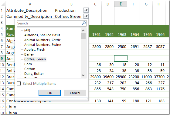
In the sheet with the pivot table we have at the top two drop down menus where we can specify which attribute and commodity to select.

image

I use this technique quite often to view large data sets.

Sunday, April 10, 2016

CSV reading in R: a value goes missing

R has the well known read.csv function. Using a data set from USDA/FAS there was a bit of a surprise:

image_thumb[1]

In the data frame df we expect that the number of different country codes is identical to the number of different country names. It isn’t. It turned out that one of the country codes is NA (Netherlands Antilles). By default this will be interpreted as a missing value (also known as NA).  The solution is to set the optional argument na.strings = NULL. What would have been the simplest approach to quickly find the problem? 

Friday, April 8, 2016

Small LP, wrong solution


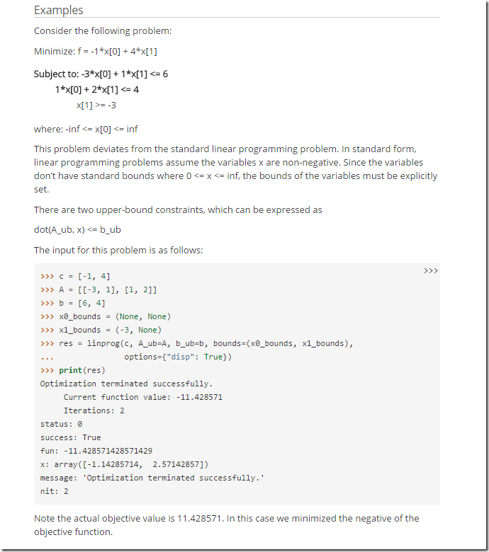
From http://docs.scipy.org/doc/scipy-0.15.1/reference/generated/scipy.optimize.linprog.html:

image

This does not look right at all.

Note: looks like this is fixed in newer versions. My python system also seems to do the right thing:

image

Thursday, April 7, 2016

MySQL Import Wizard vs LOAD INFILE

The MySQL workbench has a handy tool to import CSV files:

image

image

Unfortunately it is extremely slow. Here are some timing figures when compared with the LOAD INFILE command.

image

Timings are in seconds. Extrapolating this, it would take about 22 hours to import my 1.7 million record CSV file using the Import Wizard. I suspect this method will commit after every row, which is often a performance killer. So better use the LOAD INFILE command:

image

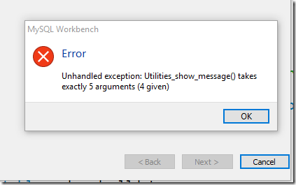
PS. Be aware that using the import wizard, the cancel button does not work during the import:

image

Tuesday, April 5, 2016

Web based visualization of multi-criteria model results

Some funding became available to add a Web based visualization tools to a larger engineering design application. Below is a depiction of the architecture. The solution points are (all or many) Pareto optimal solutions. Existing tools to visualize solutions were coded in Matlab. The new HTML and Javascript based output will allow easier dissemination of results (in addition to Excel based reports).

image

Interactive three-dimensional plots are generated using the Plotly tools.

image

Two-dimensional plots are based on Bokeh.

image

To view results with a surrogate data set click on the above figures. The HTML documents contain all data and large Javascript libraries so they take a little while to load. I am quite impressed with both Plotly and Bokeh, they offer quite some functionality. It is convenient to be able to give end-users advanced visualization capabilities without having them to install anything.