Saturday, September 30, 2017

Numberlink Models

In the Numberlink puzzle [1] we need to connect end-points by paths over a board with cells such that:

  1. Each cell is part of a path
  2. Paths do not cross

E.g. the puzzle on the left has a solution as depicted on the right [1]:


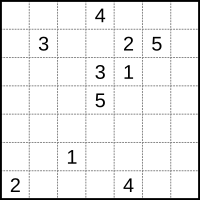
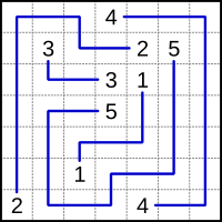
The picture on the left provides the end-points. The solution in the picture on the right can be interpreted as:

image

The main variable we use is:

\[x_{p,k} = \begin{cases}1 & \text{ if cell $p$ has value $k$}\\
                                       0 & \text{ otherwise}\end{cases}\]

The main thought behind solving this model as a math programming model is to look at the neighbors of a cell. The neighbors are the cells immediately on the left, on the right, below or above. If a cell is an end-point of a path then it has exactly one neighbor with the same value. If a cell is not an end-point it is on a path between end-points and has two neighboring cells with the same value.

image

This leads to the following high-level MIQCP (Mixed Integer Quadratically Constrained Model):

\[\bbox[lightcyan,10px,border:3px solid darkblue] {\begin{align}
                      &\sum_k x_{p,k} = 1\\
                      &\sum_{q|N(p,q)} \sum_k x_{p,k}\cdot x_{q,k} =\begin{cases} 1&\text{if cell $p$ is an end-point}\\ 2&\text{otherwise}\end{cases}\\
&x_{p,k} = c_{p,k} \>\>\> \text{if cell $p$ is an end-point}\\&x_{p,k}\in \{0,1\}\end{align}}\]

Here \(N(p,q)\) is true if \(p\) and \(q\) are neighbors and \(c_{p,k}\) indicates if cell \(p\) is an end-point with value \(k\). The model has no objective: we are just looking for a feasible integer solution. Unfortunately, this is a non-convex model. The global solver Baron can solve this during its initial local search heuristic phase:

  Doing local search
  Solving bounding LP
  Starting multi-start local search
  Done with local search
===========================================================================
    Iteration    Open nodes         Time (s)    Lower bound      Upper bound
  *         1             0            23.09      0.00000          0.00000   
            1             0            23.11      0.00000          0.00000   

  Cleaning up

                         *** Normal completion ***           

  Wall clock time:                    23.73
  Total CPU time used:                23.12

  Total no. of BaR iterations:       1
  Best solution found at node:       1
  Max. no. of nodes in memory:       1

  All done

Of course we can try to linearize this model so it becomes a MIP model (and thus convex). The product of two binary variables \(y=x_1\cdot x_2\) can be linearized by:

\[\begin{align}
&y \le x_1\\
&y\le x_2\\
&y \ge x_1+x_2-1\\
&y \in \{0,1\}\end{align}\]

We can relax \(y\) to a continuous variable between 0 and 1. In our model we can exploit some symmetry. This reduces the number of variables and equations:

\[\begin{align}
&y_{p,q,k} \le x_{p,k}&\forall p<q\\
&y_{p,q,k} \ge x_{p,k}+x_{q,k}-1&\forall p<q\\
&y_{p,q,k} \in \{0,1\}&\forall p<q\end{align}\]

The non-linear counting equation can now be written as:

\[\sum_{q|N(p,q)}  \sum_k \left( y_{p,q,k}|p<q + y_{q,p,k}|q<p \right)= b_{p}\]

Here \(b_p\) is the right-hand side of the counting constraint. This solves very fast. Cplex shows:

Tried aggregator 2 times.
MIP Presolve eliminated 6178 rows and 1840 columns.
MIP Presolve modified 40 coefficients.
Aggregator did 394 substitutions.
Reduced MIP has 11167 rows, 3892 columns, and 26610 nonzeros.
Reduced MIP has 3892 binaries, 0 generals, 0 SOSs, and 0 indicators.
Presolve time = 0.19 sec. (42.60 ticks)
Found incumbent of value 0.000000 after 0.36 sec. (79.41 ticks)

Root node processing (before b&c):
   Real time             =    0.36 sec. (79.70 ticks)
Sequential b&c:
   Real time             =    0.00 sec. (0.00 ticks)
                           ------------
Total (root+branch&cut) =    0.36 sec. (79.70 ticks)
MIP status(101): integer optimal solution
Cplex Time: 0.36sec (det. 79.72 ticks)

Cplex solves this in the root node.

Unique solution

A well-formed puzzle has exactly one solution. We can check this by adding a constraint that forbids the solution we just found. After adding this cut the model should be infeasible. Let \(\alpha_{p,k} = x^*_{p,k}\) be our feasible solution. Then our cut can look like:

\[\sum_{p,k} \alpha_{p,k} x_{p,k} \le |P|-1\]

where \(|P|\) is the number of cells. Indeed, when we add this constraint, the model becomes infeasible. So, we can conclude this is a proper puzzle.

Alternative formulation

In the comments Rob Pratt suggests a formulation that works a better in practice. The counting constraint is replaced by:

\[\begin{align}
&\sum_{q|N(p,q)} x_{q,k}=1 &&\text{if cell $p$ is an end-point with value $k$}\\
&2x_{p,k}\le \sum_{q|N(p,q)} x_{q,k} \le 2x_{p,k}+M_p(1-x_{p,k})&&\text{if cell $p$ is not an end-point}
\end{align}\]

where \(M_p\) can be replaced by \(M_p=|N(p,q)|=\sum_{q|N(p,q)} 1\) (the number of neighbors of cell \(p\)). This is at most 4 so not really a big big-M.

This formulation seems to work better. We can solve with this something like:

image

image

This problem has also exactly one solution.

Historical note

In [3] an early version of this puzzle is mentioned, appearing in

image

image

Here the goal is to draw paths from each house to its gate without the paths overlapping [4].

Large problems

For larger problems MIP solvers are not the best tool. From notes in [2] it looks like SAT solvers are most suitable for this type problem. In a CP/SAT framework we could use directly an integer variable \(x_p \in \{1,\dots,K\}\), and write the counting constraints as something like:

\[\sum_{q|N(p,q)} 1|(x_p=x_q) = \begin{cases} 1&\text{if cell $p$ is an end-point}\\ 2&\text{otherwise}\end{cases}\]
References
  1. Numberlink, https://en.wikipedia.org/wiki/Numberlink
  2. Hakan Kjellerstrand, Numberlink puzzle in Picat, https://github.com/hakank/hakank/blob/master/picat/numberlink.pi (shows a formulation in the Picat language)
  3. Aaron Adcock, Erik D. Demaine, Martin L. Demaine, Michael P. O'Brien, Felix Reidl, Fernando Sanchez Villaamil, and Blair D. Sullivan, Zig-Zag Numberlink is NP-Complete, 2014, https://arxiv.org/pdf/1410.5845.pdf
  4. Facsimiles of The Brooklyn Daily Eagle,  http://bklyn.newspapers.com/image/50475607/, https://bklyn.newspapers.com/image/50475838/
  5. Neng-Fa Zhou, Masato Tsuru, Eitaku Nobuyama, A Comparison of CP, IP, and SAT Solvers through a common interface, 2012, http://www.sci.brooklyn.cuny.edu/~zhou/papers/tai12.pdf

Wednesday, September 27, 2017

von Koch and Z3


Replica of the Zuse Z3 [5].

In [1] we showed a MIP formulation to label a tree graph in a “graceful” way [2]. Here we use the SMT (Satisfiability Modulo Theories [3]) solver Z3 from Microsoft [4]. Z3 is a library and for this example we use the Python bindings. (Z3 is also the name of an early computer, see the picture above).

The problem can be stated as follows. Using a tree graph with \(n\) nodes and \(n-1\) arcs, assign unique integer labels \(1,\dots,n\) to the nodes and \(1,\dots,n-1\) to the arcs such that for an arc \((i,j)\) we have

\[\mathit{ArcLabel}(i,j) = |\mathit{NodeLabel}(i)-\mathit{NodeLabel}(j)|\]

We use again the small dataset:

enter image description here

On the right is one possible solution.

So our model needs to handle the following conditions:

  1. \(1 \le \mathit{NodeLabel(i)} \le n\) and all-different
  2. \(1 \le \mathit{ArcLabel(i,j)} \le n-1\) and all-different
  3. \(\mathit{ArcLabel}(i,j) = |\mathit{NodeLabel}(i)-\mathit{NodeLabel}(j)|\)

The Z3 model is fairly high-level, and we can model these conditions quite naturally.

from z3 import *

nodes = ['a','b','c','d','e','f','g']

network = [('a','b'),('a','d'),('a','g'),
          ('b','c'),('b','e'),
          ('e','f')]

numnodes = len(nodes)
numarcs = len(network)

# nodes
X = [ Int('%s' % nodes[i]) for i in range(numnodes) ]

X_AllDifferent = Distinct( [ X[i] for i in range(numnodes) ] )
X_LB = And( [ X[i] >= 1 for i in range(numnodes) ] ) 
X_UB = And( [ X[i] <= numnodes for i in range(numnodes) ] ) 
X_cons = [ X_AllDifferent,X_LB,X_UB ]

# arcs
A = [ Int('%s.%s' % network[i]) for i in range(numarcs) ]

A_AllDifferent = Distinct( [ A[i] for i in range(numarcs) ] )
A_LB = And( [ A[i] >= 1 for i in range(numarcs) ] ) 
A_UB = And( [ A[i] <= numarcs for i in range(numarcs) ] ) 
A_cons = [ A_AllDifferent,A_LB,A_UB ]

# get node numbers of arcs
node1 = [nodes.index(network[i][0]) for i in range(numarcs)]
node2 = [nodes.index(network[i][1]) for i in range(numarcs)]

# no built-in absolute value
def Abs(x):
    return If(x >= 0,x,-x)

# difference
XA_cons = And([ A[i] == Abs(X[node1[i]]-X[node2[i]]) for i in range(numarcs) ])

all_cons = X_cons + A_cons + [ XA_cons ] 

solve(all_cons)

The main issue is that Z3 does not have a built-in Abs function. So, we implement our Abs using an If.

The output looks like:

[f = 5,
 b = 2,
 a = 7,
 c = 6,
 d = 1,
 e = 3,
 g = 4,
 e.f = 2,
 b.e = 1,
 b.c = 4,
 a.g = 3,
 a.d = 6,
 a.b = 5]
Enumerating all solutions

Like a MIP solver Z3 returns just one solution. We can enumerate all solutions by adding a constraint that forbids the current solution. For the above solution such a constraint can look like Or[f!=5,b!=2,a!=7,c!=6,d!=1,e!=3,g!=4]. A complete algorithm is:

s = Solver()
s.add(all_cons)
k = 0
res = []
while s.check() == sat:
    m = s.model()
    k = k + 1
    sol = [m.evaluate(X[i]) for i in range(numnodes)]
    res = res + [(k,sol)]
    forbid = Or([X[i] != sol[i] for i in range(numnodes)])
    s.add(forbid)     
print(res)

Indeed we also get our 52 solutions (only the node labels are reproduced here):

[(1, [4, 1, 6, 5, 7, 3, 2]), (2, [1, 5, 2, 6, 3, 4, 7]), (3, [1, 5, 2, 7, 3, 4, 6]), 
(4, [2, 7, 5, 3, 1, 4, 6]), (5, [1, 7, 4, 2, 3, 5, 6]), (6, [2, 6, 4, 5, 1, 7, 3]),
(7, [7, 3, 6, 1, 5, 4, 2]), (8, [7, 3, 6, 2, 5, 4, 1]), (9, [7, 1, 4, 6, 5, 3, 2]),
(10, [6, 1, 3, 5, 7, 4, 2]), (11, [7, 1, 3, 4, 5, 6, 2]), (12, [7, 1, 3, 2, 5, 6, 4]),
(13, [7, 1, 4, 2, 5, 3, 6]), (14, [7, 2, 4, 1, 5, 6, 3]), (15, [7, 2, 4, 3, 5, 6, 1]),
(16, [6, 2, 4, 5, 7, 1, 3]), (17, [6, 2, 4, 3, 7, 1, 5]), (18, [5, 1, 4, 6, 7, 2, 3]),
(19, [4, 1, 5, 6, 7, 2, 3]), (20, [3, 1, 5, 6, 7, 2, 4]), (21, [3, 1, 5, 4, 7, 2, 6]),
(22, [4, 1, 5, 3, 7, 2, 6]), (23, [2, 1, 6, 5, 7, 3, 4]), (24, [2, 1, 6, 4, 7, 3, 5]),
(25, [6, 1, 3, 2, 7, 4, 5]), (26, [4, 1, 6, 2, 7, 3, 5]), (27, [5, 1, 4, 3, 7, 2, 6]),
(28, [5, 7, 3, 2, 1, 6, 4]), (29, [5, 2, 6, 3, 7, 1, 4]), (30, [2, 6, 4, 3, 1, 7, 5]),
(31, [3, 7, 4, 2, 1, 6, 5]), (32, [1, 6, 4, 7, 3, 2, 5]), (33, [6, 7, 2, 3, 1, 5, 4]),
(34, [1, 7, 5, 6, 3, 2, 4]), (35, [3, 6, 2, 5, 1, 7, 4]), (36, [1, 6, 2, 7, 5, 3, 4]),
(37, [1, 6, 4, 5, 3, 2, 7]), (38, [1, 7, 5, 4, 3, 2, 6]), (39, [1, 6, 2, 4, 5, 3, 7]),
(40, [5, 2, 6, 4, 7, 1, 3]), (41, [3, 7, 4, 5, 1, 6, 2]), (42, [7, 2, 6, 1, 3, 5, 4]),
(43, [7, 2, 6, 4, 3, 5, 1]), (44, [3, 6, 2, 4, 1, 7, 5]), (45, [4, 7, 3, 2, 1, 6, 5]),
(46, [2, 7, 5, 6, 1, 4, 3]), (47, [1, 7, 4, 6, 3, 5, 2]), (48, [4, 7, 2, 3, 1, 5, 6]),
(49, [4, 7, 3, 5, 1, 6, 2]), (50, [5, 7, 3, 4, 1, 6, 2]), (51, [4, 7, 2, 6, 1, 5, 3]),
(52, [6, 7, 2, 4, 1, 5, 3])]

The last model was infeasible and caused the loop to end. We can in fact print this model and see how all the cuts where added:

[Distinct(a, b, c, d, e, f, g),
 And(a >= 1, b >= 1, c >= 1, d >= 1, e >= 1, f >= 1, g >= 1),
 And(a <= 7, b <= 7, c <= 7, d <= 7, e <= 7, f <= 7, g <= 7),
 Distinct(a.b, a.d, a.g, b.c, b.e, e.f),
 And(a.b >= 1,
     a.d >= 1,
     a.g >= 1,
     b.c >= 1,
     b.e >= 1,
     e.f >= 1),
 And(a.b <= 6,
     a.d <= 6,
     a.g <= 6,
     b.c <= 6,
     b.e <= 6,
     e.f <= 6),
 And(a.b == If(a - b >= 0, a - b, -(a - b)),
     a.d == If(a - d >= 0, a - d, -(a - d)),
     a.g == If(a - g >= 0, a - g, -(a - g)),
     b.c == If(b - c >= 0, b - c, -(b - c)),
     b.e == If(b - e >= 0, b - e, -(b - e)),
     e.f == If(e - f >= 0, e - f, -(e - f))),
 Or(a != 4, b != 1, c != 6, d != 5, e != 7, f != 3, g != 2),
 Or(a != 1, b != 5, c != 2, d != 6, e != 3, f != 4, g != 7),
 Or(a != 1, b != 5, c != 2, d != 7, e != 3, f != 4, g != 6),
 Or(a != 2, b != 7, c != 5, d != 3, e != 1, f != 4, g != 6),
 Or(a != 1, b != 7, c != 4, d != 2, e != 3, f != 5, g != 6),
 Or(a != 2, b != 6, c != 4, d != 5, e != 1, f != 7, g != 3),
 Or(a != 7, b != 3, c != 6, d != 1, e != 5, f != 4, g != 2),
 Or(a != 7, b != 3, c != 6, d != 2, e != 5, f != 4, g != 1),
 Or(a != 7, b != 1, c != 4, d != 6, e != 5, f != 3, g != 2),
 Or(a != 6, b != 1, c != 3, d != 5, e != 7, f != 4, g != 2),
 Or(a != 7, b != 1, c != 3, d != 4, e != 5, f != 6, g != 2),
 Or(a != 7, b != 1, c != 3, d != 2, e != 5, f != 6, g != 4),
 Or(a != 7, b != 1, c != 4, d != 2, e != 5, f != 3, g != 6),
 Or(a != 7, b != 2, c != 4, d != 1, e != 5, f != 6, g != 3),
 Or(a != 7, b != 2, c != 4, d != 3, e != 5, f != 6, g != 1),
 Or(a != 6, b != 2, c != 4, d != 5, e != 7, f != 1, g != 3),
 Or(a != 6, b != 2, c != 4, d != 3, e != 7, f != 1, g != 5),
 Or(a != 5, b != 1, c != 4, d != 6, e != 7, f != 2, g != 3),
 Or(a != 4, b != 1, c != 5, d != 6, e != 7, f != 2, g != 3),
 Or(a != 3, b != 1, c != 5, d != 6, e != 7, f != 2, g != 4),
 Or(a != 3, b != 1, c != 5, d != 4, e != 7, f != 2, g != 6),
 Or(a != 4, b != 1, c != 5, d != 3, e != 7, f != 2, g != 6),
 Or(a != 2, b != 1, c != 6, d != 5, e != 7, f != 3, g != 4),
 Or(a != 2, b != 1, c != 6, d != 4, e != 7, f != 3, g != 5),
 Or(a != 6, b != 1, c != 3, d != 2, e != 7, f != 4, g != 5),
 Or(a != 4, b != 1, c != 6, d != 2, e != 7, f != 3, g != 5),
 Or(a != 5, b != 1, c != 4, d != 3, e != 7, f != 2, g != 6),
 Or(a != 5, b != 7, c != 3, d != 2, e != 1, f != 6, g != 4),
 Or(a != 5, b != 2, c != 6, d != 3, e != 7, f != 1, g != 4),
 Or(a != 2, b != 6, c != 4, d != 3, e != 1, f != 7, g != 5),
 Or(a != 3, b != 7, c != 4, d != 2, e != 1, f != 6, g != 5),
 Or(a != 1, b != 6, c != 4, d != 7, e != 3, f != 2, g != 5),
 Or(a != 6, b != 7, c != 2, d != 3, e != 1, f != 5, g != 4),
 Or(a != 1, b != 7, c != 5, d != 6, e != 3, f != 2, g != 4),
 Or(a != 3, b != 6, c != 2, d != 5, e != 1, f != 7, g != 4),
 Or(a != 1, b != 6, c != 2, d != 7, e != 5, f != 3, g != 4),
 Or(a != 1, b != 6, c != 4, d != 5, e != 3, f != 2, g != 7),
 Or(a != 1, b != 7, c != 5, d != 4, e != 3, f != 2, g != 6),
 Or(a != 1, b != 6, c != 2, d != 4, e != 5, f != 3, g != 7),
 Or(a != 5, b != 2, c != 6, d != 4, e != 7, f != 1, g != 3),
 Or(a != 3, b != 7, c != 4, d != 5, e != 1, f != 6, g != 2),
 Or(a != 7, b != 2, c != 6, d != 1, e != 3, f != 5, g != 4),
 Or(a != 7, b != 2, c != 6, d != 4, e != 3, f != 5, g != 1),
 Or(a != 3, b != 6, c != 2, d != 4, e != 1, f != 7, g != 5),
 Or(a != 4, b != 7, c != 3, d != 2, e != 1, f != 6, g != 5),
 Or(a != 2, b != 7, c != 5, d != 6, e != 1, f != 4, g != 3),
 Or(a != 1, b != 7, c != 4, d != 6, e != 3, f != 5, g != 2),
 Or(a != 4, b != 7, c != 2, d != 3, e != 1, f != 5, g != 6),
 Or(a != 4, b != 7, c != 3, d != 5, e != 1, f != 6, g != 2),
 Or(a != 5, b != 7, c != 3, d != 4, e != 1, f != 6, g != 2),
 Or(a != 4, b != 7, c != 2, d != 6, e != 1, f != 5, g != 3),
 Or(a != 6, b != 7, c != 2, d != 4, e != 1, f != 5, g != 3)]
References
  1. The von Koch conjecture, http://yetanothermathprogrammingconsultant.blogspot.com/2017/09/the-von-koch-conjecture.html
  2. Graceful Labeling, https://en.wikipedia.org/wiki/Graceful_labeling
  3. Satisfiability modulo theories, https://en.wikipedia.org/wiki/Satisfiability_modulo_theories
  4. https://github.com/Z3Prover/z3
  5. Z3 (computer), https://en.wikipedia.org/wiki/Z3_(computer)

Thursday, September 21, 2017

The von Koch conjecture

Helge von Koch.jpg
Helge von Koch (1870-1924)

Consider a tree graph \(G=(V,E)\) with \(n\) nodes and \(n-1\) arcs. We can label the nodes with unique numbers \(1,\dots,n\) and the arcs with unique numbers \(1,\dots,n-1\) such that each arc has a label equal to the (absolute value) of difference of the labels of the attached nodes. This is also called “Graceful Labeling” [1].

Here is a picture from [2]:

enter image description here

We see that:

  • Each node has a unique label between 1 and 7 (the black numbers),
  • Each arc has a unique label between 1 and 6 (the red numbers),
  • Each arc has a label value equal to the difference in the labels of the associated nodes.

In [3] an interesting MIP formulation is proposed to find such a graceful labeling. There is no objective, i.e. we just look for a feasible solution. The uniqueness of node and arc labels is established by using an assignment block using binary variables (i.e. constraints we recognize from an assignment problem). A formulation can look like:

\[ \bbox[lightcyan,10px,border:3px solid darkblue]{ \begin{align}
\text{Node labels}\\&\sum_i x_{i,v} = 1\>\>\forall v&&\text{assignments of node labels}\\
&\sum_v x_{i,v} = 1 \>\>\forall i\\
&v^x_i  = \sum_v v \cdot x_{i,v}&&\text{value of node labels}\\
\hline
\text{Arc labels}\\&\sum_{(i,j)\in E} y_{i,j,e} = 1\>\forall e&&\text{assignment of arc labels}\\
&\sum_e  y_{i,j,e} = 1 \>\>\forall (i,j)\in E\\
&v^y_{i,j}  = \sum_e e \cdot y_{i,j,e}&&\text{value of arc labels}\\
\hline
\text{Relate arc/node}\\&v^y_{i,j} = | v^x_i - v^x_j | \>\>\forall (i,j)\in E&&\text{absolute value}&\\
\hline
\text{Variables}\\&x_{i,v} \in \{0,1\}&&\text{assign label $v$ to node $i$} \\
&y_{i,j,e} \in \{0,1\}&&\text{assign label $e$ to arc $(i,j)$}\\
&v^x_i \in \{1,\dots,n\}&&\text{value of node labels}\\
&v^y_{i,j} \in \{1,\dots,n-1\}&&\text{value of arc labels}
\end{align}} \]

It makes sense to form the set \(E\) only with arcs \(i<j\) to prevent duplication (if we have an arc \(a \rightarrow b\) we don’t want to check also \(b \rightarrow a\)).

The absolute value equation still needs to be linearized, which we detail next.

Linearizing the absolute value

A standard formulation for \(y=|x|\) uses “\(y= -x\) or \(y=x\)”, i.e.

\[\begin{align} & –x – \delta M \le y \le –x + \delta M\\
& x –(1-\delta) M \le y \le x + (1-\delta) M\\&\delta \in \{0,1\} \end{align} \]

We can slightly improve, by using:

\[\begin{align} & –x \le y \le –x + \delta M\\
& x \le y \le x + (1-\delta) M\\&\delta \in \{0,1\} \end{align} \]

For our model we can get good values for the big-M's:

\[\begin{align}
&v^y_{i,j} \ge v^x_i - v^x_j\\
&v^y_{i,j} \ge v^x_j - v^x_i\\
&v^y_{i,j} \le v^x_j - v^x_i  + 2 n \delta_{i,j} \\
&v^y_{i,j} \le v^x_j - v^x_j  + 2 n (1-\delta_{i,j}) \\
& \delta_{i,j} \in \{0,1\}
\end{align}\]

This is the formulation presented in [3]. The solution is not unique. I see:

----     74 VARIABLE vx.L  node labels

a 7,    b 1,    c 4,    d 2,    e 5,    f 3,    g 6


----     74 VARIABLE vy.L  arc labels

            b           c           d           e           f           g

a           6                       5                                   1
b                       3                       4
e                                                           2

This is different from the solution in the picture.

Alternatives?

It seems tempting to try using an alternative approach to the absolute value constraint. May be something like:

\[\begin{align}\min\>&\sum_{(i,j)\in E} v^y_{i,j}\\
&v^y_{i,j} \ge v^x_i - v^x_j\\
&v^y_{i,j} \ge v^x_j - v^x_i\end{align}\]

These formulations do not work (in this case the objective is actually constant and does not really drive down the individual \(v^y\)’s).

Enumerate solutions

We already established that the solution is not unique. How many solutions are there for this small example problem?

We can add a simple cut:

\[\sum_{i,v} \alpha_{i,v} x_{i,v} \le n-1\]

where \(\alpha_{i,v}=x^*_{i,v}\)  is a previously found solution. This will forbid this solution to be found again. If we solve again we will either find a new, different solution, or we see the model has become infeasible. In the latter case we can conclude there are no more solutions to be found. 

If we repeat this, we find a surprisingly large number of solutions (I expected to see a dozen or so). Below are the node and arc labels we collected in the solve loop:

----    124 PARAMETER vxall  collected node labels

              a           b           c           d           e           f           g

k1            7           1           4           2           5           3           6
k2            5           7           3           4           1           6           2
k3            1           6           4           5           3           2           7
k4            3           6           2           4           1           7           5
k5            7           3           6           2           5           4           1
k6            1           7           5           4           3           2           6
k7            1           5           2           7           3           4           6
k8            6           2           4           5           7           1           3
k9            7           2           4           3           5           6           1
k10           2           7           5           6           1           4           3
k11           4           7           3           2           1           6           5
k12           3           7           4           2           1           6           5
k13           2           1           6           5           7           3           4
k14           4           7           3           5           1           6           2
k15           7           3           6           1           5           4           2
k16           6           1           3           2           7           4           5
k17           7           2           6           4           3           5           1
k18           5           1           4           3           7           2           6
k19           5           1           4           6           7           2           3
k20           6           7           2           3           1           5           4
k21           1           6           2           4           5           3           7
k22           7           2           6           1           3           5           4
k23           1           6           4           7           3           2           5
k24           1           6           2           7           5           3           4
k25           4           7           2           3           1           5           6
k26           7           1           4           6           5           3           2
k27           7           2           4           1           5           6           3
k28           5           7           3           2           1           6           4
k29           7           1           3           4           5           6           2
k30           1           7           5           6           3           2           4
k31           4           1           5           3           7           2           6
k32           3           7           4           5           1           6           2
k33           1           5           2           6           3           4           7
k34           3           6           2           5           1           7           4
k35           4           1           6           2           7           3           5
k36           2           7           5           3           1           4           6
k37           4           1           5           6           7           2           3
k38           1           7           4           6           3           5           2
k39           6           1           3           5           7           4           2
k40           6           7           2           4           1           5           3
k41           4           7           2           6           1           5           3
k42           6           2           4           3           7           1           5
k43           2           1           6           4           7           3           5
k44           4           1           6           5           7           3           2
k45           7           1           3           2           5           6           4
k46           5           2           6           3           7           1           4
k47           3           1           5           6           7           2           4
k48           5           2           6           4           7           1           3
k49           2           6           4           3           1           7           5
k50           3           1           5           4           7           2           6
k51           1           7           4           2           3           5           6
k52           2           6           4           5           1           7           3


----    124 PARAMETER vyall  collected arc labels

            a.b         a.d         a.g         b.c         b.e         e.f

k1            6           5           1           3           4           2
k2            2           1           3           4           6           5
k3            5           4           6           2           3           1
k4            3           1           2           4           5           6
k5            4           5           6           3           2           1
k6            6           3           5           2           4           1
k7            4           6           5           3           2           1
k8            4           1           3           2           5           6
k9            5           4           6           2           3           1
k10           5           4           1           2           6           3
k11           3           2           1           4           6           5
k12           4           1           2           3           6           5
k13           1           3           2           5           6           4
k14           3           1           2           4           6           5
k15           4           6           5           3           2           1
k16           5           4           1           2           6           3
k17           5           3           6           4           1           2
k18           4           2           1           3           6           5
k19           4           1           2           3           6           5
k20           1           3           2           5           6           4
k21           5           3           6           4           1           2
k22           5           6           3           4           1           2
k23           5           6           4           2           3           1
k24           5           6           3           4           1           2
k25           3           1           2           5           6           4
k26           6           1           5           3           4           2
k27           5           6           4           2           3           1
k28           2           3           1           4           6           5
k29           6           3           5           2           4           1
k30           6           5           3           2           4           1
k31           3           1           2           4           6           5
k32           4           2           1           3           6           5
k33           4           5           6           3           2           1
k34           3           2           1           4           5           6
k35           3           2           1           5           6           4
k36           5           1           4           2           6           3
k37           3           2           1           4           6           5
k38           6           5           1           3           4           2
k39           5           1           4           2           6           3
k40           1           2           3           5           6           4
k41           3           2           1           5           6           4
k42           4           3           1           2           5           6
k43           1           2           3           5           6           4
k44           3           1           2           5           6           4
k45           6           5           3           2           4           1
k46           3           2           1           4           5           6
k47           2           3           1           4           6           5
k48           3           1           2           4           5           6
k49           4           1           3           2           5           6
k50           2           1           3           4           6           5
k51           6           1           5           3           4           2
k52           4           3           1           2           5           6

Note that there are \(7!=5040\) ways to order seven different labels, so from that perspective this is indeed a small subset of feasible node labels.

Instead of doing this solve loop ourselves we can also use the Solution Pool technology available in some solvers such as Cplex and Gurobi. This automates this loop (and does it way smarter and more efficient).

References
  1. Graceful Labeling, https://en.wikipedia.org/wiki/Graceful_labeling
  2. The von Koch conjecture, https://codegolf.stackexchange.com/questions/119263/the-von-koch-conjecture
  3. Mike Appleby, https://github.com/appleby/graceful-tree
  4. Helge von Koch, https://en.wikipedia.org/wiki/Helge_von_Koch
  5. Barbara M. Smith, Jean-Francois Puget, Constraint Models for graceful graphs, Constraints (2010), vol. 15, pp.64-92, https://link.springer.com/article/10.1007/s10601-009-9071-6. This paper discusses some interesting alternative models when attacking this as a Constraint Programming problem.

Monday, September 18, 2017

Conference Scheduler

In [1,2] a Python-based conference scheduler is presented. The problem is as follows:

  • There are events (i.e. talks) denoted by \(i\) and slots denoted by \(j\)
  • Some restrictions include:
    • Do not schedule talks by the same speaker at the same slot
  • Assign events to slots such that one of the following objectives is optimized:
    • Minimize total room overflow (that is: demand exceeds capacity)
    • Minimize maximum room overflow
    • Minimize changes from previous schedule

In [2] the model is stated as follows:

\[\bbox[lightcyan,10px,border:3px solid darkblue]{ \begin{align}
\min\>&\sum_{i,j} (d_i-c_j) x_{i,j}&&\text{Sum of room overflow}\\
          &\sum_j x_{i,j} =1\>\forall i \\
          &\sum_i x_{i,j} \le 1\>\forall j \\
          &x_{i,j} = 0\> \forall i,j \in C_S && \text{Unavailability} \\
          &x_{i,j} + x_{i’,j’} \le 1\> \forall i,j,i’,j’ \in C_E &&\text{Not at same day}\\
          &x_{i,j} \in \{0,1\}
\end{align}}\]

You can choose any single one from the objectives:

\[\begin{align}
1.&\sum_{i,j} (d_i-c_j) x_{i,j}&&\text{Sum of room overflow}\\
2.&\max_{i,j} (d_i-c_j) x_{i,j}&&\text{Max of room overflow}\\
3.&\sum_{i,j} \left[(1-x^0_{i,j})x_{i,j}+x^0_{i,j}(1-x_{i,j})\right]&&\text{Difference from a previous solution $x^0$}
\end{align}\]

The model can be solved with a MIP solver (via the PULP Python package) or using a simulated annealing code.

This is a nice, clean model. Of course there are always things I probably would do differently, largely based on taste.

  1. When I did something like this I used a variable \(x_{e,r,t}\) with \(r,t\) indicating the room and the time period. In this package \(j\) captures both \((r,t)\). As the package supports events and slots of different length (e.g. 30, 60, 90 minutes) that makes sense.
  2. Objective 1 seems to prefer assignments with \(d_i \ll c_j\). This can be fixed by using: \(\sum_{i,j} \max(d_i-c_j,0) x_{i,j}\). Of course we can do even better by also penalizing assignments of small events to big rooms, as shown in the rightmost picture:

    image
  3. It is not always easy to choose between the sum vs the max (objectives 1 and 2). Actually often a combination works very well.
  4. Similar for the last objective. In general I combine this with the other objectives, so that we can deviate from an existing schedule if it pays off for another objective.
  5. Instead of fixing variables \(x\) to zero if assignments are forbidden (and leave it to the presolver to get rid of these variables) I like to not even generate these variables. I guess I am old-fashioned.
  6. I probably would make the model very elastic: make sure we can always produce a feasible schedule (at the cost of renting very expensive “emergency” rooms). This way we can at least see a solution instead of just a message “infeasible”.
  7. The input data in the tutorial seems to repeat much data. E.g. the room capacity is entered for each time slot. It is usually a good idea to “normalize” data: enter the “elementary” data only once.
  8. I often prefer to present results in spreadsheet tables, in hopefully a meaningful layout. That seems to work better as a communication tool than a text file:
    image 

OK, enough of the nitpicking.  In any case, interesting stuff.

References
  1. A Python tool to assist the task of scheduling a conference, https://github.com/PyconUK/ConferenceScheduler
  2. Documentation, http://conference-scheduler.readthedocs.io/en/latest/index.html

Thursday, September 14, 2017

Minimizing Standard Deviation

image

In [1] an attempt was made to model the following situation:

  • There are \(n=25\) bins (indicated by \(i\)), each with \(q_i\) parts (\(q_i\) is given).
  • There are \(m=5\) pallets. We can load up to 5 bins onto a pallet. (Note: this implies each pallet will get exactly 5 bins.) The set of pallets is called \(j\).
  • We want to minimize the standard deviation of the number of parts loaded onto a pallet.

The question of how to model the standard deviation thing comes up now and then, so let’s see how we can model this simple example.

First we notice that we need to introduce some kind of binary assignment variable to indicate on which pallet a bin is loaded:

\[x_{i,j}=\begin{cases}1 & \text{if bin $i$ is assigned to pallet $j$}\\0&\text{otherwise}\end{cases}\]

A first model can look like:

\[\bbox[lightcyan,10px,border:3px solid darkblue]{
\begin{align}\min\>& \sqrt{\frac{\sum_j (p_j-\mu)^2}{m-1}}&&\text{minimize standard deviation}\\
&\sum_j x_{i,j} = 1 \>\> \forall i && \text{assign bin $i$ exactly once}\\
&\sum_i x_{i,j} \le 5 \>\> \forall j && \text{at most 5 bins per pallet}\\
& p_j = \sum_i q_i x_{i,j}&&\text{number of parts on a pallet}\\
& \mu = \frac{\sum_j p_j}{m}&&\text{average number of parts on a pallet} \\
& x_{i,j} \in \{0,1\} \end{align} } \]

The variables \(p_j\) and \(\mu\) are (unrestricted) continuous variables (to be precise: \(p_j\) will be integer automatically).

The objective is complicated and would require an MINLP solver. We can simplify the objective as follows:

\[\min\>\sum_j (p_j-\mu)^2 \]

Now we have a MIQP model that can be solved with a number of good solvers.

It is possible to look at the spread in a different way (there is nothing sacred about the standard deviation) and come up with a linear objective:

\[\begin{align}\min\>&p_{\text{max}}-p_{\text{min}}\\
&p_{\text{max}} \ge p_j \>\>\forall j\\
&p_{\text{min}} \le p_j \>\>\forall j \end{align}\]

This is the range of the \(p_j\)’s. In practice we might even try to use a simpler approach:

\[\begin{align}\min\>&p_{\text{max}}\\
&p_{\text{max}} \ge p_j \>\>\forall j \end{align}\]

This objective will also reduce the spread although in an indirect way. To be complete I also want to mention that I have seen cases where a quadratic objective of the form:

\[\min\>\sum_j p_j^2\]

was used. Indirectly, this objective will also minimize the spread.

The original post [1] suggest to use as number of parts:

image

Obviously drawing from the Normal distribution will give us fractional values. In practice I would expect the number of parts to be a whole number. Of course if we would consider an other attribute such as weight, we could see fractional values. In the model per se, we don’t assume integer valued \(q_i\)’s so let’s stick with these numbers. We will see below this is actually quite a difficult data set (even though we only have 125 discrete variables, which makes the model rather small), and other data will make the model much easier to solve.

To reduce some symmetry in the model we can add:

\[p_j \ge p_{j-1}\]

Not only will this help with symmetry, it also makes the variable \(p\) easier to interpret in the solution. You can see this in the results below.

The two quadratic models were difficult to solve to optimality. I stopped after 1000 seconds and both were still working. Interestingly just minimizing \(\sum p_j^2\) seems to get a somewhat better solution within the 1000 second time limit: it reduces the range from 0.1 to 0.052 and the standard deviation from 0.04 to 0.02.

image

The linear models solve to global optimality quickly and get better results.

image

By using a linear approximation we can reduce the range to 0.034 and 0.038 (and the standard deviation to 0.014 and 0.016). The model that minimizes \(p_{max}-p_{min}\) seems to be the best performing: both the quality of the solution is very good and the solution time is the fastest (34 seconds).

This is an example of a model where MIQP solvers are not as fast as we want: they really fall behind their linear counterparts.

Optimality

Can we find the best standard deviation possible? We can use the following algorithm to give this a try:

  1. Solve the linear model with objective \(\min p_{max}-p_{min}\) to optimality.
  2. Solve the quadratic model with objective \(\min \sum_j (p_j-\mu)^2\) using MIPSTART.

This data set although small is still a big problem for state-of-the-art MIQP solvers around. Step 2 took hours on a small laptop (somewhat faster on a faster machine after throwing extra threads at it). This step did not improve the solution found in in step 1 but rather proved it has the best possible standard deviation. Still very poor performance for a very small model!

Dataset

The dataset we used turned out to be very difficult. If we use a different dataset for \(q_i\): integer values from a uniform distribution, we get much better performance.

Using the following data:

----     35 PARAMETER q 

bin1  13.000,    bin2  27.000,    bin3  21.000,    bin4  16.000,    bin5  16.000
bin6  14.000,    bin7  17.000,    bin8  27.000,    bin9  11.000,    bin10 20.000
bin11 30.000,    bin12 22.000,    bin13 30.000,    bin14 26.000,    bin15 12.000
bin16 23.000,    bin17 13.000,    bin18 15.000,    bin19 24.000,    bin20 19.000
bin21 17.000,    bin22 17.000,    bin23 12.000,    bin24 13.000,    bin25 22.000

the model with quadratic objective \(\min \sum_j (p_j-\mu)^2\) solves this in just 0.2 seconds to optimality (see the solution below). This model has exactly the same size as before, just different data for \(q_i\). This is one more proof that problem size (measured by number of variables and equations) is not necessarily a good indication of how difficult a problem is to solve.

image

References
  1. LPSolve API, Minimize a function of constraints, https://stackoverflow.com/questions/46203974/lpsolve-api-minimize-a-function-of-constraints

Thursday, September 7, 2017

Quantiles with Pandas

In [1] I showed how quantiles in GAMS are difficult, and how they can be calculated better in R. Here is some Python code to do the same:

import pandas as pd
df = pd.read_csv("p.csv")
q=df.groupby(['i','j']).quantile([0,.25,.5,.75,1])
print(q)
q.to_csv("q.csv")

The q data frame looks like:

                  Val
i  j                
i1 j1 0.00  18.002966
       0.25  28.242058
       0.50  33.222936
       0.75  62.736221
       1.00  85.770764
    j2 0.00   7.644259
       0.25  41.375281
       0.50  61.313381
       0.75  82.127640
       1.00  99.813645
    j3 0.00  14.017667
       0.25  16.559221
       0.50  30.775334
       0.75  38.482815
       1.00  67.223932
i2 j1 0.00  11.938737
       0.25  29.259331
       0.50  55.029177
       0.75  69.633259
       1.00  83.258388
    j2 0.00  16.857103
       0.25  28.783298
       0.50  53.358812
       0.75  65.534761
       1.00  87.373769
    j3 0.00   5.608600
       0.25  17.433855
       0.50  33.311746
       0.75  45.566497
       1.00  64.926986

This is pretty clean. Data frames can easily be read in from CSV files (see the example above) or databases.

The new GAMS Python scripting tool is not very friendly in this respect. We need to do a lot of transformations leading to a low signal-to-noise ratio:

embeddedCode Python:
   import pandas as pd
   p = list(gams.get('p', keyFormat=KeyFormat.FLAT))
   df = pd.DataFrame(p, columns=["i", "j", "k", "value"])
   print("");print("df");print(df)
   q=df.groupby(['i','j']).quantile([0,.25,.5,.75,1])
   print("q");print(q)
# q has one multi-level index
# convert to standard indices
   q2 = q.reset_index()
   print("q2");print(q2)
# to extract a set q: convert to list of strings
   qset = q2["level_2"].unique().astype('str').tolist()
   print("qset");print(qset)
   gams.set("q", qset)
# get data itself: list of tuples
   quantiles = list(zip(q2["i"],q2["j"],q2["level_2"].astype('str'),q2["value"]))
   print("quantiles");print(quantiles)
   gams.set("quantiles",quantiles)
endEmbeddedCode q,quantiles
display q,quantiles;

Note that I am trying to prevent looping over data frame rows here: all operations are on complete columns. The CSV input/output is actually much shorter and cleaner. In this code, there is really one line that does really some work; the rest can be considered as just overhead.

The GAMS interface should probably support data frames directly to overcome this “impedance mismatch.” When users need to mix and match different languages the interface should make things as easy as possible. A GAMS/Python interface that is too low level and stays too close to GAMS asks the user to be reasonably fluent in in both GAMS and Python (the intersection of knowledgeable GAMS and Python users is likely to be small), and write quite some glue-code dealing with getting data in and out. Choosing a better abstraction level would probably help here.  

References

  1. http://yetanothermathprogrammingconsultant.blogspot.nl/2017/08/quantiles.html