Minimizing Standard Deviation

In [1] an attempt was made to model the following situation:

• There are \(n=25\) bins (indicated by \(i\)), each with \(q_i\) parts (\(q_i\) is given).
• There are \(m=5\) pallets. We can load up to 5 bins onto a pallet. (Note: this implies each pallet will get exactly 5 bins.) The set of pallets is called \(j\).
• We want to minimize the standard deviation of the number of parts loaded onto a pallet.

The question of how to model the standard deviation thing comes up now and then, so let’s see how we can model this simple example.

First we notice that we need to introduce some kind of binary assignment variable to indicate on which pallet a bin is loaded:

\[x_{i,j}=\begin{cases}1 & \text{if bin $i$ is assigned to pallet $j$}\\0&\text{otherwise}\end{cases}\]

A first model can look like:

\[\bbox[lightcyan,10px,border:3px solid darkblue]{ \begin{align}\min\>& \sqrt{\frac{\sum_j (p_j-\mu)^2}{m-1}}&&\text{minimize standard deviation}\\ &\sum_j x_{i,j} = 1 \>\> \forall i && \text{assign bin $i$ exactly once}\\ &\sum_i x_{i,j} \le 5 \>\> \forall j && \text{at most 5 bins per pallet}\\ & p_j = \sum_i q_i x_{i,j}&&\text{number of parts on a pallet}\\ & \mu = \frac{\sum_j p_j}{m}&&\text{average number of parts on a pallet} \\ & x_{i,j} \in \{0,1\} \end{align} } \]

The variables \(p_j\) and \(\mu\) are (unrestricted) continuous variables (to be precise: \(p_j\) will be integer automatically).

The objective is complicated and would require an MINLP solver. We can simplify the objective as follows:

\[\min\>\sum_j (p_j-\mu)^2 \]

Now we have a MIQP model that can be solved with a number of good solvers.

It is possible to look at the spread in a different way (there is nothing sacred about the standard deviation) and come up with a linear objective:

\[\begin{align}\min\>&p_{\text{max}}-p_{\text{min}}\\ &p_{\text{max}} \ge p_j \>\>\forall j\\ &p_{\text{min}} \le p_j \>\>\forall j \end{align}\]

This is the range of the \(p_j\)’s. In practice we might even try to use a simpler approach:

\[\begin{align}\min\>&p_{\text{max}}\\ &p_{\text{max}} \ge p_j \>\>\forall j \end{align}\]

This objective will also reduce the spread although in an indirect way. To be complete I also want to mention that I have seen cases where a quadratic objective of the form:

\[\min\>\sum_j p_j^2\]

was used. Indirectly, this objective will also minimize the spread.

The original post [1] suggest to use as number of parts:

Obviously drawing from the Normal distribution will give us fractional values. In practice I would expect the number of parts to be a whole number. Of course if we would consider an other attribute such as weight, we could see fractional values. In the model per se, we don’t assume integer valued \(q_i\)’s so let’s stick with these numbers. We will see below this is actually quite a difficult data set (even though we only have 125 discrete variables, which makes the model rather small), and other data will make the model much easier to solve.

To reduce some symmetry in the model we can add:

\[p_j \ge p_{j-1}\]

Not only will this help with symmetry, it also makes the variable \(p\) easier to interpret in the solution. You can see this in the results below.

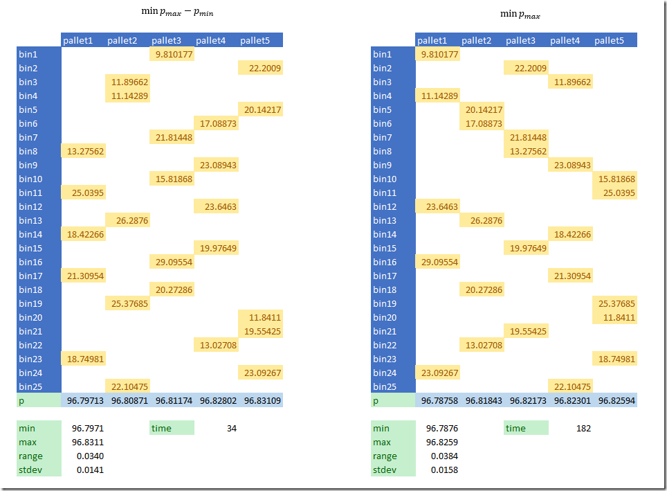
The two quadratic models were difficult to solve to optimality. I stopped after 1000 seconds and both were still working. Interestingly just minimizing \(\sum p_j^2\) seems to get a somewhat better solution within the 1000 second time limit: it reduces the range from 0.1 to 0.052 and the standard deviation from 0.04 to 0.02.

The linear models solve to global optimality quickly and get better results.

By using a linear approximation we can reduce the range to 0.034 and 0.038 (and the standard deviation to 0.014 and 0.016). The model that minimizes \(p_{max}-p_{min}\) seems to be the best performing: both the quality of the solution is very good and the solution time is the fastest (34 seconds).

This is an example of a model where MIQP solvers are not as fast as we want: they really fall behind their linear counterparts.

Optimality

Can we find the best standard deviation possible? We can use the following algorithm to give this a try:

1. Solve the linear model with objective \(\min p_{max}-p_{min}\) to optimality.
2. Solve the quadratic model with objective \(\min \sum_j (p_j-\mu)^2\) using MIPSTART.

This data set although small is still a big problem for state-of-the-art MIQP solvers around. Step 2 took hours on a small laptop (somewhat faster on a faster machine after throwing extra threads at it). This step did not improve the solution found in in step 1 but rather proved it has the best possible standard deviation. Still very poor performance for a very small model!

Dataset

The dataset we used turned out to be very difficult. If we use a different dataset for \(q_i\): integer values from a uniform distribution, we get much better performance.

Using the following data:

----     35 PARAMETER q  bin1  13.000,    bin2  27.000,    bin3  21.000,    bin4  16.000,    bin5  16.000 bin6  14.000,    bin7  17.000,    bin8  27.000,    bin9  11.000,    bin10 20.000 bin11 30.000,    bin12 22.000,    bin13 30.000,    bin14 26.000,    bin15 12.000 bin16 23.000,    bin17 13.000,    bin18 15.000,    bin19 24.000,    bin20 19.000 bin21 17.000,    bin22 17.000,    bin23 12.000,    bin24 13.000,    bin25 22.000

the model with quadratic objective \(\min \sum_j (p_j-\mu)^2\) solves this in just 0.2 seconds to optimality (see the solution below). This model has exactly the same size as before, just different data for \(q_i\). This is one more proof that problem size (measured by number of variables and equations) is not necessarily a good indication of how difficult a problem is to solve.

References

1. LPSolve API, Minimize a function of constraints, https://stackoverflow.com/questions/46203974/lpsolve-api-minimize-a-function-of-constraints