Getting rid of fly ash from coal-fired power plants

Fly ash is a by-product of coal burning power plants.

Fly ash at Cockenzie Power Station. Image by Richard Webb.

In (1) a model is presented where a group of six Chinese power plants tries to optimally sell and ship fly ash to different markets. The leftover fly ash needs to be disposed of at a certain cost. Typically disposal means using landfills. A well-known use of fly ash is as a replacement for portland cement in producing concrete. Fly ash can make the concrete stronger and more durable (2). The plants are operating under single ownership so they coordinate their actions: there is no competitive behavior between the plants and we are interested to optimize the total profit of the group.

Bricks made from Fly Ash. Image by Thamizhpparithi Maari.

The model and the paper are not very interesting. The model is rather simple, the English text in the paper is often difficult to follow and I believe the model is not correctly categorized as a Goal Programming and Scheduling Model (it is neither a scheduling model nor a goal programming model). The LP model in (1) is just:



Here \(x_{i,j}\) is a non-negative variable indicating the optimal shipping patterns from plant \(i\) to market \(j\), and \(y_i\) is the amount of fly ash we needed to dispose of. The total output of each plant is \(q_i\). Note that market price \(p_j\) and the demand are given. This is essentially a transportation model plus a little bit of logic to handle the split between selling and disposal. The results are:




This is where the paper (1) stops. However I think we can make something more interesting out of this.

Although the disposal cost are relatively small compared to the overall revenue and profit, an economist would tell you we can do better than this. By lowering the price we can increase demand and thus be able to reduce the amount we need to dispose of. In the following we will set up a scenario to see if this economist is correct. Let’s say that the demand responds to a price decrease according to a fixed price elasticity \(\eta<0\). I.e. we have:

\[\frac{\partial \ln d_j}{\partial \ln p_j} = \eta\]

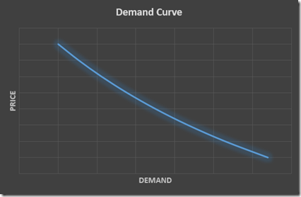
An example demand curve can look like the picture below. Although the demand curve is expressing demand as a function of price: \(d = f(p)\), economists typically make graphs with the price \(p\) on the \(y\)-axis and the quantity \(d\) on the \(x\)-axis. 

We assume here a constant price elasticity. This will result in a nonlinear demand curve. In the model we can now use the variables \(p_j\) to calculate the demand:

\[d_j = \beta_j \cdot p_j^{\eta} \]

The constant \(\beta_j\) can be found by plugging in our original constants for the price and the demand (this is called “calibration”). I.e.:

\[\beta_j := \frac{d^0_j}{(p^0_j)^\eta}\]

Assuming we don’t want to increase prices on existing customers we have: \(p_i \le p^0_j\). Quite the opposite: we want to lower prices in exchange for additional demand. Let’s further assume \(\eta = –2\) i.e. a 1% decrease in price leads to a 2% increase in demand. The model now looks like:

Note that prices (and thus the derived demand) are now endogenous instead of exogenous. As this is now an NLP model I would recommend to set some initial values for variables \(p\) and \(x\) (these are the non-linear variables). The results are:

So I would recommend to send some salespeople to markets 4, 6 and 8 and see if in exchange for a price drop the buyers are willing to purchase more. As an incentive, some of the profit improvement can be used as a bonus for these sales teams.

Of course if markets start to trade between them, this scheme may need some refinement. Another question: what about this \(\eta=-2\) elasticity? What if \(\eta=-1\) or \(\eta=-0.5\)? I ran these cases, and for \(\eta=-1\) we get rid of a some but not all disposal. The profit increases by a smaller amount than with \(\eta=-2\). With \(\eta=-0.5\) we don’t see any change compared to the original model (we have the same amount of ash to dispose of, and obtain the same profit).

References

1. Ming Fu, Lu Wang, Yong-Lan Xu, Dong-Xiao Niu, Tian-Nan Ma,"The Study of Fly Ash Scheduling Optimization Model in Coal-Fired Power Plant". In Steven Y. Liang, Energy and Mechanical Engineering, Proceedings of 2015 International Conference on Energy and Mechanical Engineering.
2. http://flyash.com/about-fly-ash/