A difficult row selection problem

The problem

In [1] an interesting problem is posted. From a matrix \(A_{i,j}\) (\(i=1,\dots,m\),\(j=1,\dots,n\)) select \(K\) rows such that a cost function is minimized. Let \(S\) be the set of selected rows. The cost function is defined as: \[ \min_S \> \left\{ 0.2 \max_{i \in S} A_{i,1} + 0.4 \sum_{i \in S} A_{i,2} - 0.3 \sum_{i \in S} A_{i,3} - 0.1 \max_{i \in S} A_{i,4} \right\} \] This problem is by no means simple to model (probably unbeknownst to the poster). Let's dive in.

Selecting rows

We define a binary decision variable:
\[\delta_i = \begin{cases} 1 &\text{if row $i$ is selected}\\ 0 &\text{otherwise}\end{cases}\]
We want to select \(K\) rows:
\[\sum_i \delta_i = K \]

A simpler objective

If the cost function was just  \[ \min_S \> \left\{ 0.4 \sum_{i \in S} A_{i,2} - 0.3 \sum_{i \in S} A_{i,3} \right\} \] things are easy. We can write: \[\min\>  0.4 \sum_i \delta_i A_{i,2} - 0.3 \sum_i \delta_i A_{i,3}\]

As this cost function is separable in the rows, we can even use simple algorithm to solve problem (instead of using a MIP mode):

1. Create a vector \(c_i =  0.4 A_{i,2} - 0.3 A_{i,3}\)
2. Sort the vector \(c\) 
3. Pick rows that correspond to the \(K\) smallest values of \(c\)

The \(\max\) terms in the objective make the objective non-separable in the rows, so this little algorithm is no longer applicable.

Review: Modeling a maximum

The maximum \(z = \max(x,y)\) where \(x\) and \(y\) are decision variables, can in general be modeled as: \[\bbox[lightcyan,10px,border:3px solid darkblue]{\begin{align} &z\ge x\\ &z \ge y\\ &z \le x + M \eta\\ & z\le y + M(1-\eta)\\ &\eta \in \{0,1\}\end{align}}\]

Here \(M\) is a large enough constant. This formulation can be interpreted as: \[\begin{align}&z \ge x \text{ and } z \ge y\\  &z \le x \text{ or } z \le y \end{align}\]

The maximum of a set of variables: \(z = \max_k x_k\) is a direct extension of the above: \[\bbox[lightcyan,10px,border:3px solid darkblue]{\begin{align} &z\ge x_k && \forall k\\  &z \le x_k + M \eta_k&& \forall k\\ & \sum_k \eta_k = 1\\ &\eta_k \in \{0,1\}\end{align}}\] This formulation is correct in all cases. We can simplify things a little bit depending on how the objective is written.

If we are minimizing the maximum we can actually simplify things considerably:\[\min \left\{\max_k x_k \right\} \Rightarrow \begin{cases}\min &z\\ &z \ge x_k & \forall k\end{cases}\]

Maximizing the maximum does not save much. We can write:
\[
\max \left\{  \max_k  x_k \right\}  \Rightarrow \begin{cases}\max   & z\\& z \le x_k+M \eta_k & \forall k\\ & \displaystyle \sum_k \eta_k = 1\\ &\eta_k \in \{0,1\}
\end{cases}\]

A complete model

We generate a small data set with 10 rows. We want to select \(K=2\) rows that maximize our objective. The data part of the model can look like: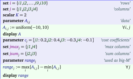

The model itself using the most general implementation of the maximum can look like:

Notes:

• The parameter range functions as a big-M constant.
• The variables \(\eta_{i,j}\) are only used for the \(j\)'s corresponding to a "max" column.
• We needed to make sure that the selected row with the maximum (i.e. \(\eta_{i,j}=1\)) is limited the selected rows. We do this by requiring \(\delta_j=0 \Rightarrow \eta_{i,j}=0\).
• We can simplify things for the first objective where \(c_j>0\). For this column we have a simple "minimax" case. This means we can drop equations maxObj2, sum1, and implyZero and the corresponding \(\eta\)'s from the model. We still need them for the last column.
• Similarly we can drop equation maxObj1 when  \(c_j < 0\) (objective 4).
• An optimized model can therefore look like:
  
  
  
  
  
  

The results look like:

----     57 PARAMETER A  data

             j1          j2          j3          j4

i1       -6.565       6.865       1.008      -3.977
i2       -4.156      -5.519      -3.003       7.125
i3       -8.658       0.004       9.962       1.575
i4        9.823       5.245      -7.386       2.794
i5       -6.810      -4.998       3.379      -1.293
i6       -2.806      -2.971      -7.370      -6.998
i7        1.782       6.618      -5.384       3.315
i8        5.517      -3.927      -7.790       0.048
i9       -6.797       7.449      -4.698      -4.284
i10       1.879       4.454       2.565      -0.724


----     57 VARIABLE delta.L  select rows

i3 1.000,    i5 1.000


----     57 VARIABLE obj.L  single objectives

j1 -6.810,    j2 -4.994,    j3 13.341,    j4  1.575


----     57 VARIABLE z.L                   =       -7.519  final objective

The solution can also be viewed as:

The data set is small enough to enumerate all possible solutions. There are only 45 different ways to select two rows from ten, so we can just select the best objective:

As an aside, the different configurations were generated by letting the solution pool technology in Cplex enumerate all solutions to the optimization problem: \[ \begin{align} \min\>&0\\ & \sum_i x_i = K\\ & x_i \in \{0,1\} \end{align} \] This explains the somewhat strange ordering of the different solutions. Of course this overkill: if you have a hammer in the form of a solver, everything looks like an optimization problem.

A larger data set with \(m=10,000\) rows and \(K=100\) took 30 seconds to solve even though it has 20,000 binary variables. The number of combinations for this problem is \[{{m}\choose{K}} = \frac{m!}{(m-K)!K!} \] This is a big number for these values:

65208469245472575695415972927215718683781335425416743372210247172869206520770178988927510291340552990847853030615947098118282371982392705479271195296127415562705948429404753632271959046657595132854990606768967505457396473467998111950929802400

A little bit too big to try complete enumeration.

References

1. https://stackoverflow.com/questions/48098198/choose-optimal-subset-of-size-k-given-certain-constraints-r