Monday, January 30, 2017

Little trick: random positive definite matrix

Sometimes we want to test a model with some random data. When dealing with quadratic problems we may need to invent a positive definite matrix \(Q\). One simple way to do this is as follows:

image

I.e. in matrix terms: \(Q:=Q^TQ\) (i.e. the assignment above is not done one-by-one but rather in parallel). To be precise: \(Q\) will be positive semi-definite, i.e. \(x^TQx\ge 0\).

This simple device can help generating random data for convex quadratic models.

Thursday, January 26, 2017

MIP modeling: Selecting subsets

Consider the following problem, original from (1):

We have a population of items with values having a mean \(\mu\). Furthermore we have a number of subsets of this population. Each subset \(i\) has a known count \(n_i\) and mean \(\mu_i\). It can be assumed the subsets do not overlap: the pairwise intersection between two subsets is always empty. We want to select \(N\) subsets such that the total average of all selected items is as close to \(\mu\) as possible.

OK, let’s see. Let:

\[\delta_i = \begin{cases}1 & \text{if subset $i$ is selected}\\
                                   0 & \text{otherwise}\end{cases}\]

We could model the problem as:

\[\boxed{\begin{align} \min \> & \left| \mu – \frac{\sum_i n_i \mu_i \delta_i}{\sum_i n_i \delta_i} \right|\\
    & \sum_i \delta_i = N \\
    & \delta_i \in \{0,1\} \end{align}} \]

where \(|.|\) indicates `absolute value`.

The objective is somewhat complicated. The ratio is the average of the items in the selected subsets. We can see this as follows. The average is the sum of the values of the items in the selected subsets divided by the number if selected items. Of course, the sum of values in a subset \(i\) is \(n_i \mu_i\) which explains the numerator in the fraction.

This model is quite nonlinear, but there is a way to linearize this. The first thing we can do is introduce a variable \(y\) defined by

\[y=\frac{\sum_i n_i \mu_i \delta_i}{\sum_i n_i \delta_i}\]

and reformulate as:

\[ \sum_i n_i (y \delta_i ) = \sum_i n_i \mu_i \delta_i\]

This is nonlinear because of the multiplication \(y\cdot\delta_i\). However, a multiplication of a binary variable and a continuous variable can be linearized with a little bit of effort (2). Let’s introduce a new variable \(x_i = y \cdot \delta_i\), then we can form the linear inequalities:

\[\begin{align}
    &y^{LO} \cdot \delta_i \le x_i \le y^{UP} \cdot \delta_i\\
    &y-y^{UP}\cdot (1-\delta_i) \le x_i \le y-y^{LO}\cdot (1-\delta_i)
\end{align}\]

Here \(y^{LO},y^{UP}\) is the lower- and upper-bound on \(y\). We can use:

\[\begin{align} &y^{LO} := \min_i \mu_i\\
&y^{UP} := \max_i \mu_i \end{align}\]

With this we can rewrite the condition \(\sum_i n_i (y \delta_i) = \sum_i n_i \mu_i \delta_i\) as:

\[\sum_i n_i x_i = \sum_i n_i \mu_i \delta_i\]

The absolute value can be handled in a standard way, e.g.:

\[\begin{align} \min\>& z\\
                              &-z \le \mu – y \le z \end{align}\]

Now we have all the tools to write the complete linear model:

\[\boxed{\begin{align}
      \min\>& z\\
               &-z \le \mu – y \le z \\
                  &y^{LO} \cdot \delta_i \le x_i \le y^{UP} \cdot \delta_i\\
    &y-y^{UP}\cdot (1-\delta_i) \le x_i \le y-y^{LO}\cdot (1-\delta_i) \\
    &\sum_i n_i x_i = \sum_i n_i \mu_i \delta_i\\
    & \sum_i \delta_i = N \\
    & \delta_i \in \{0,1\} \\
    & z \ge 0 \\
    & y^{LO} \le y \le y^{UP} \\
    & x_i \>\text{free}
\end{align}}\]

What if the subsets can overlap? That means a data element \(a_k\) can be a member of multiple subsets. If we want it to be counted just once, we need to consider the data elements themselves. This implies the need to introduce a binary variable that indicates whether \(a_k\) is in any of the selected subsets. I believe the high-level model can look like:

\[\boxed{\begin{align}
    \min\> & \left| \mu – \frac{\sum_k a_k \alpha_k}{\sum_k \alpha_k} \right|\\
              & \alpha_k = \prod_i s_{i,k} \delta_i\\
              & \sum_i \delta_i = N \\
              & \delta_i, \alpha_k \in \{0,1\}
\end{align}}\]

Here we have data: \(s_{i,k}=1\) if value \(a_k\) is in subset \(i\). This can be linearized in a similar fashion. 

References
  1. http://stackoverflow.com/questions/41879502/find-subset-with-similar-mean-as-full-set
  2. Multiplication of a continuous and a binary variable, http://yetanothermathprogrammingconsultant.blogspot.com/2008/05/multiplication-of-continuous-and-binary.html

Tuesday, January 24, 2017

Employee Scheduling III: generating all shifts using the Cplex solution pool

In (1) and (2) all possible shifts for a small Employee Scheduling problem are calculated by programming. In (3) we generate new shifts one by one using MIP model as part of a Column Generation algorithm. Here I want to show a different approach to generate all possible feasible shifts with a MIP model using the Cplex solution pool. So this is a post about “modeling instead of programming”.

The model is very similar to the sub-problem in the Column Generation scheme:

binary variables
   w(t)
'work at time t'
   start(t)
'start of shift'
   emp(e)
'select shift from employee e'
;
positive variables
   shiftlen 
'length of shift'
;
variable dummy;

equations

   startShift(t)   
'start of shift: w(t) goes from 0 to 1'
   oneShiftStart   
'exactly one start of shift'
   calcLen         
'calculate length of shift'
   oneEmployee     
'pick one employee'
   minLength       
'observe minimum shift length'
   maxLength       
'observe maximum shift length'
   feasibleShift(t)
'make sure shift is feasible'
   dummyObj
;

startShift(t)..  start(t) =g= w(t) - w(t--1);
oneShiftStart.. 
sum(t,start(t)) =e= 1;
calcLen..        shiftLen =e=
sum
(t, w(t));
oneEmployee..   
sum
(e, emp(e)) =e= 1;
minLength..      shiftLen =g=
sum
(e, minlen(e)*emp(e));
maxLength..      shiftLen =l=
sum
(e, maxlen(e)*emp(e));
feasibleShift(t).. w(t) =l=
sum
(canwork(e,t),emp(e));
dummyObj..       dummy =e= 0;


option
mip=cplex;

$onecho > cplex.opt
SolnPoolAGap = 0.0

SolnPoolIntensity = 4
PopulateLim = 10000
SolnPoolPop = 2
solnpoolmerge solutions.gdx
$offecho

model solpool /all/;
solpool.optfile=1;
solve
solpool using mip minimizing dummy;

Actually the model is quite simpler as in the CG sub-problem we needed a rather complicated objective. Here we use a dummy objective as we just need to find a feasible shift.

This model finds a shift encoded by the binary variable \(w_t\) and a corresponding employee denoted by \(emp_e \in \{0,1\}\) (the selected employee will have a value of one).

The start of a shift is easily found: we need to look for a pattern \(w_t,w_{t+1} = 0, 1\). Note that \(w_1\) for \(t=1\) is special: it may be a continuation of a shift with \(w_{24}=1\). This is the reason why in the GAMS model we use “start(t) =g= w(t) - w(t--1)” with a circular lag operator --. To make sure shifts are contiguous we only need to require that \(\sum_t start_t \le 1\) (note that \(\sum_t start_t = 0\) can not happen, so we can also write \(\sum_t start_t = 1\)).

We check if a shift is only using allowed time slots in equation feasibleShift. Here we use the set canwork(e,t) indicating which time periods are allowed or forbidden for a given employee (see (2)). We require here that if canwork=0 then the corresponding \(w_t=0\).

The Cplex solution pool (4) allows us to find all feasible integer solutions for a MIP very fast. This technology is used here to find all feasible shifts and indeed we find:

image

We see we find the same 1295 shifts, although in a different order (the order is not important for our purposes).

Now we have found this complete collection of feasible shifts, we can solve our scheduling model:

\[\begin{align}\min\>&\sum_s c_s x_s\\
       &\sum_{s|E(e,s)} x_s \le 1 \>\forall e\\
       &\sum_{s|S(s,t)} x_s \ge R_t \> \forall t\\
        &x_s \in\{0,1\}\end{align}\]

With this approach we just use one MIP solve to find all feasible shifts and a second MIP solve to find the optimal schedule.

References

  1. Loren Shure, Generating an Optimal Employee Work Schedule Using Integer Linear Programming, January 6, 2016, http://blogs.mathworks.com/loren/2016/01/06/generating-an-optimal-employee-work-schedule-using-integer-linear-programming/ describes the problem with a Matlab implementation.
  2. Employee Scheduling I : Matlab vs GAMS, http://yetanothermathprogrammingconsultant.blogspot.com/2017/01/employee-scheduling-i-matlab-vs-gams.html has a GAMS version of the model in (1).
  3. Employee Scheduling II : Column Generation, http://yetanothermathprogrammingconsultant.blogspot.com/2017/01/employee-scheduling-ii-column-generation.html
  4. IBM, What is the solution pool?, http://www.ibm.com/support/knowledgecenter/SSSA5P_12.7.0/ilog.odms.cplex.help/CPLEX/UsrMan/topics/discr_optim/soln_pool/02_soln_pool_defn.html
  5. Employee Scheduling IV: direct optimization, http://yetanothermathprogrammingconsultant.blogspot.com/2017/03/employee-scheduling-iv-direct.html

Monday, January 23, 2017

Employee Scheduling II: column generation

In (1) and (2) an Employee Scheduling model is considered where all possible shifts are enumerated before we solve the actual model. Although such models models tend to solve quickly (especially considering their size), generating all possible shifts may not be an option for larger problems. One possible way to attack this problem is using a traditional column generation approach. This method will generate attractive candidate solutions and add them to the problem.

Our original problem was:

\[\begin{align}\min\>&\sum_s c_s x_s\\ &\sum_{s|E(e,s)} x_s \le 1 \>\forall e\\ &\sum_{s|S(s,t)} x_s \ge R_t \>\forall t\\ &x_s \in\{0,1\}\end{align}\]

where

\[x_s = \begin{cases}1 & \text{if shift $s$ is selected}\\  0 & \text{otherwise} \end{cases}\]

Instead of generating all possible shifts in advance, we start with a small initial set \(s \in S\). We want this initial set to form a feasible solution for the problem. To make this easier we rewrite the problem as:

\[\begin{align}
\min\> & \sum_s c_s x_s + \sum_t c_t s_t\\ &\sum_{s|E(e,s)} x_s \le 1\>\forall e\\ &\sum_{s|S(s,t)} x_s + s_t \ge R_t\>\forall t \\ &x_s \in\{0,1\}\\ & s_t \ge 0\end{align}\]

Here \(s_t\) is a slack with a penalty \(c_t\). We also can consider this as extra, flexible, hourly personnel to hire at a hourly rate of \(c_t\) to cover staffing shortages. Sometimes we call this scheme: making the model “elastic”.

The column generation algorithm iterates between two different problems. First we have a master problem that is essentially a relaxed version of the elastic model we just discussed. We replace the condition \(x_s \in \{0,1\}\) by \(x_s \in [0,1]\). Using this we now have an LP (and thus we can generate duals). Second, there is a sub problem that calculates a candidate column (or candidate shift). 

image  

The sub problem uses a particular objective: it minimizes the reduced cost of the new LP column \(A_j\) wrt to the master problem. I.e. the objective is basically

\[\min \sigma_j = c_j – \pi^T A_j\]

where \(\pi\) are the LP duals of the master problem.

This scheme is called column generation as we increase the size of the number of variables \(x_s\) during the algorithm:

image

Note that the columns \(s_t\) stay fixed.

We stop iterating as soon as we can no longer find a new column with \(\sigma_j < 0\), indicating a “profitable” column. We now have collection of shifts and an LP solution. I.e. we have fractional variable values. To make this a usable schedule we need to solve one more MIP: introduce again the condition \(x_s \in\{0,1\}\). The complete algorithm can look like:

  1. Generate an initial (small) set \(S\) of feasible shifts
  2. Solve the relaxed master problem (LP)
  3. Solve the sub problem
  4. If \(\sigma_j < 0\) add shift to the set \(S\) and go to step 2
  5. Solve master problem as MIP

Initial Set

For the problem in (1) we generate 100 random feasible shifts. The first 10 shifts are as follows:

image

Note that we have here two shifts for employee White. This is no problem: the master problem will select the most suitable one to include in the schedule. All these shifts are feasible: they obey the minimum and maximum hours and will not use hours an employee is not available. If the shifts are not sufficient to cover all staffing requirements, no problem: the LP model will start hiring the expensive hourly “emergency” workers. Indeed for these 100 random shifts we need some extra hourly help:

----    214 VARIABLE short.L  staffing shortage in time t

t5  1.000,    t6  1.000,    t7  1.000,    t9  2.000,    t13 1.000,    t15 1.000,    t16 1.000,    t17 1.000
t18 1.000,    t19 1.000,    t23 1.000


Master Problem

The master problem expressed in GAMS looks like:

set
   s0
'shifts' /s1*s1000/
   s(s0)
'dynamic subset will grow during algorithm'
   esmap(e,s0)
'mapping between employee and shift'
   shifts(s0,t)
'data structire to hold shifts'
;

parameters
   a(t,s0)
'matrix growing in dimension s'
   c(s0)  
'cost vector growing in dimension s'
;

scalar
   shortcost
'cost to hire extra hourly staff' /200/
;

binary variable x(s0) 'main variable: shift is selected';
positive variable short(t) 'staffing shortage in time t'
;
variable
cost;

equations

  masterObj       
'calculate total cost'
  oneShift(e)     
'each employee can do at most one shift'
  coverPeriod(t)  
'cover each period'
;

masterObj..
   cost =e=
sum(s, c(s)*x(s)) + sum(t,shortcost*short(t));

oneShift(e)..
  
sum
(esmap(e,s), x(s)) =l= 1;

coverPeriod(t)..
  
sum
(shifts(s,t), x(s)) + short(t) =g= requirements(t);

model Master /masterObj,oneShift,coverPeriod/
;


Sub problem

The sub problem is somewhat more difficult. We need to find a feasible shift and minimize the reduced cost \(\sigma_j\).

set sh 'feasible shift hours' /sh2*sh8/;
parameter
shlen(sh);
shlen(sh) =
ord
(sh)+1;

binary variables

   w(t)
'work at time t'
   start(t)
'start of shift'
   emp(e)
'select shift from employee e'
   shft(sh)
'select feasible shift length'
   se(sh,e)
'select (sh,e) combination'
;
variables
   shiftlen 
'length of shift'
   wagecost
   redcost  
'reduced cost'
;

equations
   startShift(t)   
'start of shift: w(t) goes from 0 to 1'
   oneShiftStart   
'exactly one start of shift'
   calcLen         
'calculate length of shift'
   oneEmployee     
'pick one employee'
   minLength       
'observe minimum shift length'
   maxLength       
'observe maximum shift length'
   feasibleShift(t)
'make sure shift is feasible'
   calcShift1      
'select shift length'
   calcShift2      
'id'
   secomb(sh,e)    
'shift/employee combination'
   calcwage        
'calculate cost of shift'
   subObj          
'objective'
;

startShift(t)..  start(t) =g= w(t) - w(t--1);
oneShiftStart.. 
sum(t,start(t)) =e= 1;
calcLen..        shiftLen =e=
sum
(t, w(t));
oneEmployee..   
sum
(e, emp(e)) =e= 1;
minLength..      shiftLen =g=
sum
(e, minlen(e)*emp(e));
maxLength..      shiftLen =l=
sum
(e, maxlen(e)*emp(e));
feasibleShift(t).. w(t) =l=
sum
(canwork(e,t),emp(e));
calcShift1..    
sum
(sh,shft(sh)) =e= 1;
calcShift2..    
sum
(sh,shlen(sh)*shft(sh)) =e= shiftlen;
secomb(sh,e)..   se(sh,e) =g= shft(sh) + emp(e) - 1;
calcwage..       wageCost =e=
sum
((sh,e),shlen(sh)*wage(e)*se(sh,e));
subObj..
  redcost =e= wageCost -
sum(e,emp(e)*oneShift.m(e)) - sum
(t, w(t)*coverPeriod.m(t));
model sub /subObj,startShift,oneShiftStart,calcLen,oneEmployee,minLength,

          
maxLength,feasibleShift,calcShift1,calcShift2,secomb,calcWage/
;


Some of the modeling issues with the sub problem are explained in more detail in (3).

Column Generation Algorithm

The CG algorithm itself can look like:

sets
  iter
/iter1*iter100/
;

scalars
   continue
/1/
;
parameter
   masterObjVal(iter)
;

loop(iter$continue,

  
solve
master using rmip minimizing cost;
   masterObjVal(iter) = cost.L;

  
solve
sub using mip minimizing redcost;

  
if
(redcost.l < -0.001,
      esmap(e,nexts)$(emp.l(e)>0.5) =
yes
;
      shifts(nexts,t)$(w.l(t)>0.5) =
yes
;
      c(nexts) = wagecost.L;
      s(nexts) =
yes
;
      nexts(s0) = nexts(s0-1);
  
else

     continue = 0;
   );

);

solve
master using mip minimizing cost;


Results

We need to do 36 cycles before we can conclude there are no more interesting columns. The objective of the relaxed master problem decreases to an LP objective representing a cost of $4670. Of course the LP objective is non-increasing: adding a column (i.e. adding a shift) can only help.

image

After these 36 iterations we have collected 135 shifts (remember we starting in the first iteration with our 100 randomly generated initial shifts). This compares quite favorably to the 1295 shifts we obtained by enumerating all possible shifts. When we reintroduce the integer restrictions \(x_s\in \{0,1\}\) the objective value deteriorates to $4675. This is just a little bit worse than the global optimal objective of $4670. Indeed this method does not guarantee to find absolute best integer solution, however often it finds very good solutions.

The final schedule looks like:

image

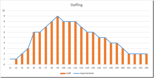
We don’t need any expensive hourly “emergency” staff, i.e. \(s_t = 0\). Again we have no slack in the system: we precisely meet the staffing requirements every hour:

image


References

  1. Loren Shure, Generating an Optimal Employee Work Schedule Using Integer Linear Programming, January 6, 2016, http://blogs.mathworks.com/loren/2016/01/06/generating-an-optimal-employee-work-schedule-using-integer-linear-programming/ describes the problem with a Matlab implementation.
  2. Employee Scheduling I: Matlab vs GAMS, http://yetanothermathprogrammingconsultant.blogspot.com/2017/01/employee-scheduling-i-matlab-vs-gams.html has a GAMS version of the model in (1).
  3. Employee Scheduling III: generating all shifts using the Cplex solution pool, http://yetanothermathprogrammingconsultant.blogspot.com/2017/01/employee-scheduling-iii-generating-all.html
  4. Erwin Kalvelagen, Column Generation with GAMS, http://www.amsterdamoptimization.com/pdf/colgen.pdf has some background on Column Generation in GAMS.
  5. Employee Scheduling IV: direct optimization, http://yetanothermathprogrammingconsultant.blogspot.com/2017/03/employee-scheduling-iv-direct.html

Friday, January 20, 2017

Employee Scheduling I: Matlab vs GAMS

In (1) a small employee scheduling problem is modeled as a simple MIP model using MATLAB. Basically from the data on employee availability, we need to form all possible shifts. Even for small data sets that can become a large number. Having all these possible shifts we introduce a binary variable:  

\[x_s = \begin{cases}1 & \text{if shift $s$ is selected}\\
                              0 & \text{otherwise} \end{cases}\]

We have some requirements with respect to staffing levels, and an employee can only do one shift in the 24 hours we are look at. The standard model for this is:

\[\begin{align}\min\>&\sum_s c_s x_s\\
                            &\sum_{s|E(e,s)} x_s \le 1\>\forall e\\
                            &\sum_{s|S(s,t)} x_s \ge R_t \> \forall t\\
                            &x_s \in\{0,1\}\end{align}\]

The first constraint says each employee can perform at most one shift. The second constraint makes sure that we have enough shifts selected such that we meet staffing requirements. The objective minimizes the cost associated with the selected shifts. This is a very simple model, so actually the main issues are with data manipulation: we need to form a collection of all possible shifts.

Data

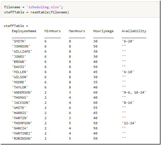
We reproduce here the data from (1):
image

Data entry using Excel is always very convenient. Most users know and have access to Excel. Notice that the last column  (Availability) is a string, which needs to be parsed inside the application.  Matlab has sscanf, GAMS has no similar facilities. If you want to directly read this into GAMS you could use 4 columns, say Start1, End1, Start2, End2 with integer values.

The staffing requirements are:

image

Matlab code

The Matlab code from (1) and (2) combines generating the shifts and producing the LP matrix. This makes it more difficult to understand the model: it is hidden inside the code. I quickly scanned the code, but decided not to translate this into GAMS but rather start from scratch. Translating code line-by-line is often not as useful.

The blog post (1) displays the non-zero pattern of the LP matrix. In my opinion, in a GAMS environment such a picture is not very useful.

GAMS code: generating shifts

The GAMS code I wrote separates generation of shifts from the model equations. As it turns out the first task is not completely trivial.

The first thing I did was to generate a set canwork(e,t) containing whether a time slot is allowed by an employee:

image

This was produced from the rules:

canwork(e,t)$(data(e,'start1')=0 and data(e,'end1')=0) = yes;
canwork(e,t)$(
ord(t)>data(e,'start1') and ord(t)<=data(e,'end1')) = yes
;
canwork(e,t)$(
ord(t)>data(e,'start2') and ord(t)<=data(e,'end2')) = yes
;

The next thing I did was to generate a parameter maxstart(e,t) indicating how long the maximum shift can be starting in period t. This looks something like:

image

It is not simple to compute. Note that near the end of the day we still can start a long shift: shifts wrap from t24 to t1. Here is my code:

set back(t,tt) 'used to loop backwards over time';
back(t,tt)$(
ord(tt)+ord(t)=card(t)+1) = yes
;
* when looping over this set tt runs backwards

parameters
   count0(e,t)   
'max length of remaining part of shift in t1'
   maxstart(e,t) 
'max length of shift starting in t'
;

*
* First calculate maximum length of remaining part of shift in t1
* This is used when wrapping from t24 to t1.
* Notes:
*   We scan backwards.
*   count0(e,t) is indexed by t, but we only use t=t1.
*
count0(e,t) = 0;
loop(back(t,tt),
   count0(e,
't1')$canwork(e,tt) = min(count0(e,'t1'
)+1,maxlen(e));
   count0(e,
't1')$(not
canwork(e,tt)) = 0;
);

*

* Now calculate maximum length of shift starting in t
*
maxstart(e,t) = 0;
loop
(back(t,tt),
   maxstart(e,tt)$canwork(e,tt) = min(maxstart(e,tt+1)+1+count0(e,t),maxlen(e));
);
maxstart(e,tt)$(maxstart(e,tt)<minlen(e)) = 0;


From this we can compute the following:

  1. The set shifts(s,t) with a shift id s and hour t.
  2. A mapping set esmap(e,s), that maps between employee e and shift s.
  3. A subset s of used shifts.

The data structure shifts looks like:

image

We can see here just a part of the shifts. There are 1295 of them. Near the bottom we see a few shifts wrapping from t24 to t1.

Shifts s1 through s24 belongs to employee Smith; Johnson owns shifts s25-s96. This correspondence is stored in the mapping set esmap(e,s). The code to generate this is:

sets
  s0
'shifts'  /s1*s10000/
  s(s0)
'used shifts'
  k(s0)
/s1/
;
scalar i;
loop
((e,t)$maxstart(e,t),
  
for
(i = minlen(e) to maxstart(e,t),
      shifts(k,tt)$(
ord(tt)>=ord(t) and ord(tt)<ord(t)+i) = yes
;
      shifts(k,tt)$(
ord(tt)>=1 and ord(tt)<ord(t)-card(t)+i) = yes
;
      esmap(e,k) =
yes
;
      s(k) =
yes
;
      k(s0) = k(s0-1);
   );
);

Boy this was not straightforward, and the code is not very intuitive. But we managed. Probably using a standard programming language this shift generation step may be easier.

A very different technique is to use an optimization model in combination with the Cplex solution pool technology to generate all possible shifts. In (4) this approach is applied to this problem.

GAMS code: MIP model

Finally we need to implement optimization model. This is actually very easy now:

parameter shiftlen(s0) 'number of hours in a shift';
shiftlen(s) =
sum
(shifts(s,t),1);

binary variable
x(s0);
variable
cost;

equations

   oneShift(e)    
'each employee can do at most one shift'
   coverPeriod(t) 
'cover each period'
   calcCost       
'calculate total cost'
;

oneShift(e)..
  
sum(esmap(e,s), x(s)) =l= 1;

coverPeriod(t)..
  
sum
(shifts(s,t), x(s)) =g= requirements(t);

calcCost..
  cost =e=
sum
(esmap(e,s),  wage(e)*shiftlen(s)*x(s));

model m /all/
;
option optcr=0;
solve
m minimizing cost using mip;

This model follows very closely the mathematical model presented at the beginning of this post. This model solves very fast. Cplex can find the optimal solution (proving optimality) without doing any branching. The problem with this formulation is that it can generate a ton of possible shifts, but an advantage is that it often solves very fast. The results are:

image

This is different from what is shown in (1) but with the same objective: the cost is $4670. As in (1) there is no slack: we precisely match the staffing requirements:

image

References

  1. Loren Shure, Generating an Optimal Employee Work Schedule Using Integer Linear Programming, January 6, 2016, http://blogs.mathworks.com/loren/2016/01/06/generating-an-optimal-employee-work-schedule-using-integer-linear-programming/
  2. http://blogs.mathworks.com/images/loren/2016/makeMILPMatrices.m contains the matrix generation code.
  3. Employee Scheduling II : Column Generation, http://yetanothermathprogrammingconsultant.blogspot.com/2017/01/employee-scheduling-ii-column-generation.html uses a Column Generation approach to solve this problem.
  4. Employee Scheduling III : generating all shifts using the Cplex solution pool, http://yetanothermathprogrammingconsultant.blogspot.com/2017/01/employee-scheduling-iii-generating-all.html uses the Cplex Solution Pool technology to generate all possible shifts. This is an alternative approach to the method shown in this post.
  5. Employee Scheduling IV: direct optimization, http://yetanothermathprogrammingconsultant.blogspot.com/2017/03/employee-scheduling-iv-direct.html