Yet Another Math Programming Consultant: Employee Scheduling IV: direct optimization

In (1) a small employee scheduling problem is proposed. It is solved by first generating all possible shifts for each employee, and then solving a very simple MIP (Mixed Integer Programming) model to select the optimal combination of employees and shifts.

The optimization model is organized around a binary variable $x_s \in \{0,1\}$ defined by:

\[x_s = \begin{cases}1 & \text{if shift $s$ is selected}\\ 0 & \text{otherwise} \end{cases}\]

and is very straightforward:

\[\begin{align}\min\>&\sum_s c_s x_s\\
&\sum_{s|E(e,s)} x_s \le 1\>\forall e\\
&\sum_{s|S(s,t)} x_s \ge R_t \> \forall t\\ &x_s \in\{0,1\}\end{align}\]

Here $E(e,s)$ indicates if shift $s$ is done by employee $e$, $S(s,t)$ indicates if time period $t$ is covered by shift $s$ and $R_t$ is the required staffing during period $t$. The first constraint makes sure every employee is doing at most one shift in the 24-hour planning period. The second constraint establishes that we have enough staffing in each (hourly) period. Of course we try to minimize total cost.

In (2) we replicated the model in GAMS, using GAMS code to generate all possible shifts. In (4) we used a different technique to generate all shifts: the Cplex solution pool. In (3) we don’t generate all shifts in advance, but use a delayed column generation scheme to generate attractive shifts on the fly.

Here I try to show that we can attack the problem also in a very different way: directly optimize the selection of employees to use and the hours they work. A basic model to generate a single feasible shift for this problem is shown in (4) and (3). In those (sub-)models a binary variable $w_t \in \{0,1\}$ is used to indicate if an employee is working at period $t$. For our “direct” model we extend this to:

\[w_{e,t} = \begin{cases}1 & \text{if employee $e$ works during period $t$}\\ 0 & \text{otherwise} \end{cases}\]

Again we first calculate the set canwork(e,t) indicating the time slots employee e can work. Furthermore we have parameters minlen(e) and maxlen(e) that tell us the minimum and maximum length of a shift for a given employee. Also the problem states that a shift is contiguous, i.e. no holes in the shift.

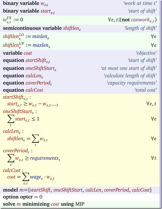
A MIP model can look like:

Notes:

We fix $w_{e,t}=0$ when canwork(e,t) is not true.
The variable shiftlen(e) is a semi-continuous variable. It can be zero, or between minlen(e) and maxlen(e).
If you don’t want to use semi-continuous variables, we can use binary variables $\delta_e$ instead, and apply the constraint:

\[\begin{align}&minlen_e \cdot \delta_e \le shiftlen_e \le maxlen_e \cdot\delta_e\\
&\delta_e \in \{0,1\}\\& shiftlen \ge 0\end{align}\]
where shiftlen is now a positive variable. In GAMS we need to split this into two inequalities.
The binary variable start(e,t) indicates when a shift starts. We observe this when w(e,t) switches from zero to one. A standard formulation is $start_{e,t} \ge w_{e,t} – w_{e,t-1}$. As we need to wrap around hour 24: hour 1 minus 1 is hour 24, we use the GAMS $—$ operator: $start_{e,t} \ge w_{e,t} – w_{e,t--1}$.
We only allow up to one start to enforce that we have no breaks in a shift: shifts are contiguous in this model.

We rely on the presolver of the MIP solver to remove all fixed variables from the model. I am old-fashioned and I prefer to not even generate the variables that are not needed. This requires a little bit of attention. The new model can look like:

binary variables
   w(e,t) 'work at time t'
   start(e,t) 'start of shift'
;

semicont variables
   shiftlen(e) 'length of shift'
;
shiftlen.lo(e) = minlen(e);
shiftlen.up(e) = maxlen(e);

variable cost 'objective';

equations
   startShift(e,t)     'start of shift'
   oneShiftStart(e)    'at most one start of shift'
   calcLen(e)          'calculate length of shift'
   coverPeriod(t)      'capacity requirements'
   calcCost            'total cost'
;

startShift(canwork(e,t))..
   start(e,t) =g= w(e,t) - w(e,t--1)$canwork(e,t--1);
oneShiftStart(e)..
   sum(canwork(e,t),start(e,t)) =l= 1;
calcLen(e)..
   shiftLen(e) =e= sum(canwork(e,t), w(e,t));
coverPeriod(t)..
   sum(canwork(e,t), w(e,t)) =g= requirements(t);
calcCost..
   cost =e= sum(canwork(e,t), wage(e)*w(e,t));

model m /all/;
option optcr=0;
solve m minimizing cost using mip;

In this model I “protected” the use of $w_{e,t}$ by canwork(e,t) in all cases. Note that in equation startShift the expression

w(e,t--1)$canwork(e,t--1) evaluates to zero when $w_{e,t—1}$ does not correspond to canwork(e,t--1) being true. That is exactly what we want: if canwork(e,t) if false, implicitly we want the corresponding $w_{e,t}=0$. We can verify the correct behavior by inspecting the equation listing in GAMS:

---- startShift =G= start of shift

startShift(SMITH,t7).. - w(SMITH,t7) + start(SMITH,t7) =G= 0 ; (LHS = 0)

startShift(SMITH,t8).. w(SMITH,t7) - w(SMITH,t8) + start(SMITH,t8) =G= 0 ; (LHS = 0)

startShift(SMITH,t9).. w(SMITH,t8) - w(SMITH,t9) + start(SMITH,t9) =G= 0 ; (LHS = 0)

REMAINING 415 ENTRIES SKIPPED

The first version of the model has the following statistics:

MODEL STATISTICS

BLOCKS OF EQUATIONS           5     SINGLE EQUATIONS          545
BLOCKS OF VARIABLES           4     SINGLE VARIABLES          981
NON ZERO ELEMENTS         3,381     DISCRETE VARIABLES        918

while the second version shows:

MODEL STATISTICS

BLOCKS OF EQUATIONS           5     SINGLE EQUATIONS          483
BLOCKS OF VARIABLES           4     SINGLE VARIABLES          857
NON ZERO ELEMENTS         2,942     DISCRETE VARIABLES        856

Results

This model solves quickly (it is small), and we find an optimal solution with a cost of 4670. The schedule looks like:

We see one shift wrapping at t24: Employee Davis. The optimal solution is not unique. In (1) and (2) different solutions are obtained (with the same total cost). The optimal solution has no slack in staffing: we exactly match the staffing requirements:

[image%255B31%255D.png]

References

- Loren Shure, Generating an Optimal Employee Work Schedule Using Integer Linear Programming, January 6, 2016, http://blogs.mathworks.com/loren/2016/01/06/generating-an-optimal-employee-work-schedule-using-integer-linear-programming/ describes the problem with a Matlab implementation.
- Employee Scheduling I: Matlab vs GAMS, http://yetanothermathprogrammingconsultant.blogspot.com/2017/01/employee-scheduling-i-matlab-vs-gams.html has a GAMS version of the model in (1).
- Employee Scheduling II : Column Generation, http://yetanothermathprogrammingconsultant.blogspot.com/2017/01/employee-scheduling-ii-column-generation.html uses a Column Generation approach to solve this problem.
- Employee Scheduling III: generating all shifts using the Cplex solution pool, http://yetanothermathprogrammingconsultant.blogspot.com/2017/01/employee-scheduling-iii-generating-all.html uses the Cplex Solution Pool technology to generate all possible shifts. This is an alternative approach to the method shown in this post.
No comments:
Post a Comment