Numbrix puzzle via TSP

 In [1], I demonstrated a small and rather elegant MIP model to solve Numbrix puzzles. Here is the comment by Austin Buchanan:

It would also be interesting to see how this compares to an MTZ-like model. And how well the two models scale to larger grids.

The Miller-Tucker-Zemlin [2,3] formulation for the Traveling Salesman Problem (TSP) starts with a standard assignment problem, and then adds some sub-tour elimination constraints. From [3]:

Note:  here \(\color{darkblue}p\ge \color{darkblue}n\). This 1960 paper has some interesting computational tests. Many runs ended with: "the machine was stopped after over 250 pivot steps had failed to produce the solution."

Numbrix puzzle via MIP

The puzzle of numbrix [1,2] is simple to state.

• We have a 9x9 board with 81 cells. 
• We need to fill each cell with a unique integer value between 1 and 81.
• There are some prefilled cells.
• We should be able to start with the cell containing value 1 and then following a path (only going one up, down, left or right) to the next values and thus eventually arriving at the cell with value 81.  

Example

Below is an example of an input (the "given" cells) and a solution. The colors may help to see that we have a path from the cell with value 1 to the cell with value 81.

Of course, we want to see if we can create a MIP model for this.

GAMS + R Markdown scripting

In [1] I discussed a small script that exported GAMS data to R for plotting. Here I expand on that and show how we can use R Markdown [2] to generate documents that contain GAMS data and results. Here we have just a small example with just a parameter. But it is easy to see that this can also be used with larger models, where we have a document built around more complex model results. 

R Markdown can handle as input text, R code, R graphics and LaTeX math (among others). Output can be HTML, PDF (via LaTeX), and DOCX (MS Word).

GAMS + R scripting

 I like to automate things. That means in practice: I write scripts. I prefer to spend a little more time to develop a script, basically for two reasons:

• A script can be executed again with little or no effort.
• A script serves as documentation. 

This helps to make things reproducible.

Here is a setup I often use for post-processing GAMS results with R. 

Modeling a simple implication

From [1]:

How to model:  

if \(\color{darkred}\delta=0\) then \(\color{darkred}x=0\) else \(\color{darkred}x=\color{darkred}x\)

where \(\color{darkred}\delta\in \{0,1\}\) is a binary variable and \(\color{darkred}x\ge 0\) is a non-negative continuous variable. 

The else part looks strange, but it is meant to indicate: unrestricted. So better is to just drop the else part:

if \(\color{darkred}\delta=0\) then \(\color{darkred}x=0\)

Let's list some possible formulations. 

Electronic Amoeba for solving TSPs?

Abstract

Combinatorial optimization to search for the best solution across a vast number of legal candidates requires the development of a domain-specific computing architecture that can exploit the computational power of physical processes, as conventional general-purpose computers are not powerful enough. Recently, Ising machines that execute quantum annealing or related mechanisms for rapid search have attracted attention. These machines, however, are hard to map application problems into their architecture, and often converge even at an illegal candidate. Here, we demonstrate an analogue electronic computing system for solving the travelling salesman problem, which mimics efficient foraging behaviour of an amoeboid organism by the spontaneous dynamics of an electric current in its core and enables a high problem-mapping flexibility and resilience using a resistance crossbar circuit. The system has high application potential, as it can determine a high-quality legal solution in a time that grows proportionally to the problem size without suffering from the weaknesses of Ising machines.

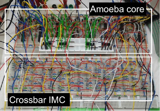
Picture of the electronic amoeba (from [2])

"Electronic amoeba" sounds awful. Furthermore, the paper talks about "legal solutions". Now the lawyers even get involved... 

 

References

1. 'Electronic amoeba' finds approximate solution to traveling salesman problem in linear time, https://www.sciencedaily.com/releases/2020/12/201210112050.htm
2. Kenta Saito, Masashi Aono and Seiya Kasai, Amoeba-inspired analog electronic computing system integrating resistance crossbar for solving the travelling salesman problem, https://www.nature.com/articles/s41598-020-77617-7

 

Directed vs undirected networks in math programming models

Many practical optimization models contain some network structures. In virtually all cases, these networks are modeled as directed graphs. I.e., between nodes \(i\) and \(j\), we consider arcs \(i \rightarrow j\) and \(j \rightarrow i\). In graph theory, it is very customary to talk about undirected graphs. In this case, there is just one link between nodes \(i\) and \(j\). Why am I using directed graphs, with two uni-directional arcs for each pair of nodes? I will try to answer this in this post.

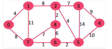
As an example, let's consider the shortest path problem. This is really the same as a min-cost problem. I took the following data (from [1]):

QuadProg: usage issues

The QuadProg QP (Quadratic Programming) solver, based on an algorithm by Goldfarb and Idnani [1,2], is quite popular. It is available for R [3] and Python [4]. However, it has some real drawbacks. Some of it is just "user interface" and documentation: how to call the solver.

The mathematical model the solver works with is [3]: \[\begin{align} \min\>& -\color{darkblue}d^T\color{darkred}b + \frac{1}{2}\color{darkred}b^T\color{darkblue}D\color{darkred}b \\ & \color{darkblue}A^T\color{darkred}b \begin{bmatrix}= \\ \ge \end{bmatrix} \color{darkblue}b_0 \end{align} \]

This immediately poses some questions:

• Variables are typically called \(\color{darkred}x\), and \(\color{darkblue}b\) is usually a constant. Why the different notation here?
  I don't know. Maybe to make sure you pay attention.
• How to handle bounds?
  The variable type the solver supports is called "free" (i.e. unrestricted). This is different than for many LP solvers, where the default variable type is positive. For non-negative variables, you need to explicitly add the constraints \(\color{darkred}b \ge 0\). Similar for other bounds.
• Why the different signs for the linear part and the quadratic part in the objective?
  I don't know.
• Why the constant \(1/2\) in the objective?
  We see this more often in QP solvers. This is because the gradient of the quadratic term \(\color{darkred}x^T\color{darkblue}Q\color{darkred}x\) is \(2\color{darkblue}Q\color{darkred}x\). The algorithm prefers to work with \(\color{darkblue}Q\color{darkred}x\) however. So in order to stay really close to the algorithm, the user is asked to multiply all quadratic coefficients \(\color{darkblue}D_{i,j}\) by 2.
• Most QP solvers call the matrix with quadratic coefficients \(\color{darkblue}Q\). Why is it called \(\color{darkblue}D\) here?
  Don't know.
• Does \(\color{darkblue}D\) have to be symmetric?  
  The documentation does not tell, but the answer is: only the diagonal and upper-triangular part of \(\color{darkblue}D\) are used. This means the matrix is assumed to be symmetric. E.g. when passing \[\color{darkblue}D = \begin{pmatrix} 1 & 0 \\ 100 & 1 \end{pmatrix}\] the solver thinks it received \[\color{darkblue}D = \begin{pmatrix} 1 & 0 \\ 0 & 1 \end{pmatrix}\]
• Can \(\color{darkblue}D\) be positive semi-definite?
  In QuadProg, \(\color{darkblue}D\) has to be strictly positive definite.
  Defnition: A matrix \(Q\) is called positive semi-definite when \(x^TQx\ge 0\) for all \(x\). It is called positive definite when \(x^TQx\gt 0\) for all \(x \ne 0\). A positive definite matrix has strictly positive eigenvalues. I.e., the smallest eigenvalue of \(\color{darkblue}D\) must be \(\lambda_{min}\gt 0\). For a positive semi-definite matrix all eigenvalues are non-negative (i.e., zero is allowed).
  The fact that QuadProg requires a strict positive definite matrix, means that all variables need to be quadratic and also that this algorithm can not solve LPs. Most QP solvers (in fact all the ones I know beyond QuadProg) only require positive semi-definite quadratic coefficient matrices. I.e., for linear variables we can use coefficients \(\color{darkblue}q_{i,j}=0\) (where \(i\) or \(j\) corresponds to a linear variable). Quadprog is stricter. The whole matrix \(\color{darkblue}D\) most be strictly positive definite. You should be aware of these restrictions. And the documentation [3] should have mentioned this.
• Can I trick QuadProg to accept linear variables?
  Yes, suppose we have 2 quadratic variables and 2 linear variables. Then form the \(\color{darkblue}D\) matrix as \[\color{darkblue}D = \begin{pmatrix} \color{darkblue}d_{1,1} &\color{darkblue}d_{1,2} & 0 & 0  \\ \color{darkblue}d_{2,1} &\color{darkblue}d_{2,2} & 0 & 0  \\ 0 & 0 &\color{darkblue} \varepsilon & 0 \\ 0 & 0 & 0 &\color{darkblue} \varepsilon \end{pmatrix}\] where \(\color{darkblue} \varepsilon\gt 0\) is a small constant. This trick would also allow us to feed the algorithm linear problems.
• Usually, solvers express linear constraints as \(\color{darkblue}A\color{darkred}x=\color{darkblue}b\). Why do we have a transposed matrix \(\color{darkblue}A^T\) here?
  I suspect this is closer to what the dual algorithm prefers. Again, making the input closer to what the solver wants.
• How to input \(\le\) constraints?
  Multiply these by \(-1\) and make them \(\ge\) constraints.

These are some of the questions I have seen in the past about QuadProg.  Hopefully, this at least demystifies some of them.

As an alternative to QuadProg, you may want to have a look at CVXR or CVXPY for modeling QPs. These tools can talk to different solvers and will apply the necessary transformations to make the model suited for the selected solver. The modeling is also a bit more natural than the matrix input for QuadProg. For non-trivial quadratic programming models, QuadProg may not be the best choice.  

References

1. D. Goldfarb and A. Idnani (1982). Dual and Primal-Dual Methods for Solving Strictly Convex Quadratic Programs. In J. P. Hennart (ed.), Numerical Analysis, Springer-Verlag, Berlin, pages 226–239.
2. D. Goldfarb and A. Idnani (1983). A numerically stable dual method for solving strictly convex quadratic programs. Mathematical Programming, 27, 1–33.
3. R package quadprog, https://cran.r-project.org/web/packages/quadprog/quadprog.pdf
4. Python package quadprog, https://pypi.org/project/quadprog/

Machine scheduling: Maintenance and maximum runlength

In [1] a problem is posed that deals with a maximum run-length (6 days) before the machine needs to be taken off-line for maintenance (1 day).  Consider the binary decision variable:

\[\color{darkred}y_t = \begin{cases} 1 & \text{if machine is online at period $t$} \\ 0 & \text{otherwise} \end{cases} \]

In [1] a scheme is proposed as follows. Introduce an integer variable \(\color{darkred}z_t\) that has the cumulative days the machine is running. Then apply the rule: 

if \(\color{darkred}z\gt 6\) then \(\color{darkred}y:=0,\color{darkred}z:=0\)

This approach needs a bit of repair to make it work for a MIP model. A MIP model can not contain assignments, and decision variables are part of a system of linear equations. I.e., all decision variables are essentially calculated at the same time (a notion which can be foreign for computer programmers who think in sequential assignment statements). We can write:\[\begin{align} & \color{darkred}y_t = 1 \Rightarrow \color{darkred}z_t  = \color{darkred}z_{t-1} + 1 \\ & \color{darkred}y_t = 0 \Rightarrow \color{darkred}z_t  = 0 \\ & \color{darkred}z_t \in \{0,\dots,6\}\end{align}\] This is in the form of implications that can be used directly with (advanced) solvers that support indicator constraints (i.e., a binary variable on the left and a linear constraint on the right). Note that we don't do anything special when \(\color{darkred}z_t\) becomes 7. We just forbid that from happening by setting an upper bound of 6. The initial value \(\color{darkblue}z_0\) is the number of periods the machine is already online at the beginning of the planning period. 

If your solver or modeling tool does not have support for indicator constraints, we can rewrite things as: \[\begin{align}& \color{darkblue}z_t^{up} := 6  \\ & \color{darkred}z_t \le \color{darkred} y_t \cdot \color{darkblue}z_t^{up}\\  & \color{darkred}z_t \le   \color{darkred}z_{t-1} + 1 \\ & \color{darkred}z_t \ge   \color{darkred}z_{t-1} + 1 - (1-\color{darkred}y_t ) \cdot (\color{darkblue}z_t^{up}+1)\\  & \color{darkred}z_t \in \{0,\dots,\color{darkblue}z_t^{up} \}\end{align}\] Here \( \color{darkblue}z_t^{up} =6\) is the upper bound on \( \color{darkred}z_t\). This formulation requires a little bit of thinking. Finally, I want to mention that \( \color{darkred}z_t\) can be declared as a continuous variable: it will be integer automatically. 

A simpler alternative formulation is to just forbid any sequence of 7 consecutive 1's for \(\color{darkred}y\). I.e. \[\color{darkred}y_t+\color{darkred}y_{t+1}+\color{darkred}y_{t+2}+\color{darkred}y_{t+3}+\color{darkred}y_{t+4}+\color{darkred}y_{t+5}+\color{darkred}y_{t+6} \le 6\] It may be easier to look backward: \[\color{darkred}y_t+\color{darkred}y_{t-1}+\color{darkred}y_{t-2}+\color{darkred}y_{t-3}+\color{darkred}y_{t-4}+\color{darkred}y_{t-5}+\color{darkred}y_{t-6} \le 6\] The terms \(\color{darkred}y_{t-k}\) can have a non-positive index \(t-k\) which means this is historic data, from before our planning period. In other words \(\color{darkblue}y_0,\color{darkblue}y_{-1},\color{darkblue}y_{-2},\dots\) is data.

Conclusion

This is a good example where we can achieve the same result using two very different approaches. It may make sense to choose the simplest formulation.

References

1. Linear Programming - Re-setting a variable based on it's cumulative count, https://stackoverflow.com/questions/64930027/linear-programming-re-setting-a-variable-based-on-its-cumulative-count

OR Scientist Job @ Amobee

The Operations Research Scientist is responsible for collaborating with the team to design and implement systems that focus on forecasting, allocating, delivering, and reporting of advertising on the internet, TV, and connected devices.  The successful candidate will utilize advanced mathematical, optimization, machine-learning, software engineering, and programming skills to solve challenging problems.

Responsibilities 

• Develop innovative mathematical programming (LP, MILP, …) solutions to run efficiently and at scale
• Develop innovative forecasts, models, algorithms, and solutions and build prototypes and production implementations
• Work cross-functionally to gather feedback and requirements from end users
• Be a key contributor to product innovation and company strategy
• Communicate technical information clearly to both technical and non-technical people

Qualifications:

• Degree in Operations Research, Mathematics, Statistics, Industrial Engineering, Mechanical Engineering, Physics, or related field;  MS/PhD strongly preferred
• 3+ years of relevant experience
• Strong experience with implementing decomposition techniques, column generation preferred.
• Strong analytical, statistical, and math abilities; Exceptional problem-solving skills
• Excellent communication skills
• Extreme attention to detail
• Ability to work as part of a team in a fast-paced environment
• Familiarity with GAMS, Gurobi/Cplex, CVX, Python, R, Java, Scala, SQL

More information: https://www.amobee.com/company/careers/senior-operation-research-scientist/