Tuesday, January 15, 2019

Preferences for houses and neighbors


In [1] the following problem was posted:

  • We have \(n\) houses (denoted by index \(j\))
  • and \(m\)  tenants (using index \(i\)).
  • Each tenant \(i\) has a certain preference for a given house. The tenant can express this by providing three preferred houses: 1 for most preferred, and 2 for second most preferred and 3 for the third preferred house.
  • Each tenant can also provide three preferred neighbors, using the same scheme: 1 for most preferred neighbor and 2 or 3 for less preferred. 

Let's try to build a model for this.

Data


The first thing is I assume \(n\ge m\): the number of houses exceeds the number of tenants. 

To make the objective work, we need to decide what score to use when a house or neighbor is not preferred. We cannot just use zero for this, as 1 is most preferred. We can use the number 4, i.e.: 1 is most preferred, through 4: not preferred and then minimize the achieved score. 

I like to use 0 as the default however. For this, I recode the preferences as 3 being the most preferred, and 0 being not preferred. Using zero as the default will lead to sparser models. 

I generated some random data with 8 tenants and 10 houses:


----     40 PARAMETER hpref  preference for house, recoded, 3=first,2=second,1=third

             house1      house2      house3      house4      house6      house7      house8      house9     house10

tenant1                       1                                   3                                   2
tenant2           1                                               2                                               3
tenant3                       1           3                                   2
tenant4                       1                                   2                                   3
tenant5                       2                       1           3
tenant6                                   1                       2                       3
tenant7           1           3                       2
tenant8                                   3                                   1           2


----     40 PARAMETER npref  preference for neighbor, recoded, 3=first,2=second,1=third

            tenant1     tenant2     tenant3     tenant4     tenant5     tenant6     tenant7     tenant8

tenant1                       2           1                                               3
tenant2                                                           1                       3           2
tenant3                       3                       2                       1
tenant4                       1                                               2           3
tenant5                       1           3                                               2
tenant6           2                       3           1
tenant7                                   3                       2           1
tenant8           1                                               3           2

The parameter npref can be interpreted as: \[\mathit{npref}_{i,i'} = \text{preference provided by tenant $i$ for having tenant $i'$ as neighbor}\] So each row should have three nonzero entries. This matrix is not symmetric. The benefit of having tenants \(i\) and \(i'\) as neighbors is \[\mathit{npref}_{i,i'}+\mathit{npref}_{i',i}\] The matrix composed of values \(\mathit{npref}_{i,i'}+\mathit{npref}_{i',i}\) is symmetric. I assume \(\mathit{npref}_{i,i}=0\), i.e. the diagonal is zero.

In the following I will consider the preferences as a cardinal utility: we can add things up. Theoretically, the preferences may be more like an ordinal utility: only comparison is defined. I will sidestep this issue to make things easier for me.

Assignment


The main variables of the model are: \[x_{i,j} = \begin{cases} 1 & \text{if tenant $i$ is assigned to house $j$} \\ 0 & \text{otherwise}\end{cases}\] The assignment constraints can look like: \[\begin{align} & \sum_j x_{i,j} = 1 & \forall i \\ & \sum_i x_{i,j} \le 1 & \forall j \end{align}\] This will be the backbone of the model.

Housing preferences


The objective related to housing preferences is simple: \[\max \> \sum_{i.j} \mathit{hpref}_{i,j} x_{i,j}\]

Neighbor preferences


The objective that deals with preferences for neighbors, is more complicated. Let's assume all houses are in one long row. Then we can write: \[\max \> \sum_{i,i',j}  (\mathit{npref}_{i,i'}+\mathit{npref}_{i',i})  x_{i,j} x_{i',j+1}\] This is a quadratic objective. As we shall see later, it can be easily linearized.

Complete model


The complete model can look like:

Quadratic model
\[\begin{align} \max \> & \color{DarkBlue} \lambda \color{DarkRed} f_1 + (1-\color{DarkBlue}\lambda) \color{DarkRed} f_2 \\ & \color{DarkRed} f_1 = \sum_{i.j} \color{DarkBlue}{ \mathit{hpref}}_{i,j} \color{DarkRed} x_{i,j} \\ & \color{DarkRed} f_2 = \sum_{i,i',j} \color{DarkBlue}{(\mathit{npref}}_{i,i'}+\color{DarkBlue}{\mathit{npref}}_{i',i}) \color{DarkRed}x_{i,j} \color{DarkRed}x_{i',j+1} \\ & \sum_j \color{DarkRed} x_{i,j} = 1 & \forall i \\ & \sum_i \color{DarkRed} x_{i,j} \le 1 & \forall j \\ & \color{DarkRed} x_{i,j} \in \{0,1\} \end{align} \]

Here \(\lambda\gt 0 \) is a weight. With \(\lambda = 0.8\) (most weight on the housing preferences) I see as solution:


----     79 VARIABLE x.L  assignment

             house2      house3      house4      house6      house7      house8      house9     house10

tenant1                                           1.000
tenant2                                                                                           1.000
tenant3                                                       1.000
tenant4                                                                               1.000
tenant5       1.000
tenant6                                                                   1.000
tenant7                               1.000
tenant8                   1.000


----     88 PARAMETER hpoints  preference points for house allocation

             house2      house3      house4      house6      house7      house8      house9     house10

tenant1                                           3.000
tenant2                                                                                           3.000
tenant3                                                       2.000
tenant4                                                                               3.000
tenant5       2.000
tenant6                                                                   3.000
tenant7                               2.000
tenant8                   3.000


----     88 PARAMETER npoints  preference points for neighbors

            tenant2     tenant3     tenant4     tenant6     tenant8

tenant1                   1.000
tenant3                                           4.000
tenant4       1.000
tenant5                                                       3.000
tenant6                               3.000


We can see that tenant3 and tenant6 are neigbors (house 7 and 8) and thus get 4 bonus points.

A solver like Cplex will be able to solve this model as given. There are some reformulations performed under the hood, as the problem as stated is actually non-convex.

Note: some other solvers will refuse this model as a quadratic equality constraint is non-convex. We can fix this by substituting out \(f_2\). Other solvers will still refuse to solve the model after this reformulation: the Q matrix is not positive definite, while some other solvers recognize this can be linearized. Convex QP/MIQP solvers are not in agreement about what constitutes an acceptable model. 

If the houses are not in a single row, the definition of a neighbor may be a bit more complicated. We can define the parameter \[\vartheta_{j,j'} = \begin{cases} 1 & \text{if houses $j$ and $j'$ (with $j'\gt j$) are neighbors}\\ 0 & \text{otherwise}\end{cases}\] and use as objective: \[\max \> \sum_{i,i',j,j'}  (\mathit{npref}_{i,i'}+\mathit{npref}_{i',i})  \vartheta_{j,j'} x_{i,j} x_{i',j'}\] It is noted that we need to watch out for double counting. Hence \(\vartheta_{j,j'}= 0\) for \(j'\le j\).

Linearization


If you only have access to a MIP solver, this problem can be easily reformulated into a linear MIP model by observing that \(y_{i,i',j} =  x_{i,j} x_{i',j+1}\) can be linearized as: \[\begin{align} & y_{i,i',j} \le x_{i,j} \\ & y_{i,i',j} \le x_{i',j+1} \\ & y_{i,i',j} \ge x_{i,j} + x_{i',j+1} - 1 \\& y_{i,i',j} \in \{0,1\} \end{align}\] Plugging this into our model yields a linear model.

 References

  1. Optimization solution / algorithm for occupying tenants in houses (combinations), https://stackoverflow.com/questions/54146767/optimization-solution-algorithm-for-occupying-tenants-in-houses-combinations

Sunday, January 6, 2019

(Pre)solving Killer Sudokus

Killer Sudoku [1] is a variant of Sudoku where an additional constraint is that cells belonging to a cage (the colored regions in the picture) add up to a given value.

Killer Sudoku (from [1])
As in standard Sudokus, we need to fill each cell with a number \(1,\dots,9\), and values in each row, column and \((3 \times 3)\) box must be unique. In addition, all values in a cage should be unique. In this puzzle we don't see that some cells already have given values: we need to fill-in all the cells. The solution for the above puzzle is:

Solution (from [1])
Using the standard decision variables for Sudoku puzzles: \[x_{i,j,k} = \begin{cases} 1 & \text{if cell $(i,j)$ has value $k$} \\ 0 & \text{otherwise}\end{cases}\] we can solve this easily with a MIP model. In the model below we use two data structures:

  • a mapping \(\mathit{amap}(a,i,j)\) between area \(a\) (an area is a row, column or box) and cells \((i,j)\): \(\mathit{amap}(a,i,j)\) is \(\mathit{true}\) if cell \((i,j)\) belongs to area \(a\), 
  • a similar mapping \(\mathit{cmap}(c,i,j)\) between a cage \(c\) and cell numbers \((i,j)\).
With this we can form a compact model:


Killer Sudoku model
\[\begin{align}
 & \sum_k \color{DarkRed} x_{i,j,k} = 1 && \forall i,j && \text{One value per cell}\\
& \sum_{i,j| \color{DarkBlue}{\mathit{amap}}(a,i,j)} \color{DarkRed} x_{i,j,k} = 1 && \forall a,k && \text{Unique values in each row, column and box} \\
& \sum_{i,j|  \color{DarkBlue}{\mathit{cmap}}(c,i,j)} \color{DarkRed} x_{i,j,k} \le 1 && \forall c,k && \text{Unique values in each cage}\\
& \sum_{i,j,k| \color{DarkBlue}{\mathit{cmap}}(c,i,j)} \color{DarkBlue} k \cdot \color{DarkRed} x_{i,j,k} = \color{DarkBlue} {\mathit{CageSum}}_c && \forall c && \text{Cell values add up to cage sum} \\
& \color{DarkRed} x_{i,j,k} \in \{0,1\}  \end{align}\]

There is no objective in this model: we are just looking for a feasible integer solution.

Implementation


The equivalent GAMS model can look like:

set
  a    
'area' /i1*i9,j1*j9,b1*b9/
  i(a) 
'rows' /i1*i9/
  j(a) 
'columns' /j1*j9/
  b(a) 
'boxes' /b1*b9/
  amap(a,i,j)
'mapping area<->cells'
  k    
'values' /1*9/
;

*
* populate amap
* rows, columns, and boxes a.k.a nonets
*
amap(i,i,j) =
yes;
amap(j,i,j) =
yes;
amap(b,i,j) =
ord(b) = 3*ceil(ord(i)/3) + ceil(ord(j)/3) - 3;
display amap;

*
* cages
*
sets
  c
'cages' /cage1*cage29/
  cmap(c,i,j) 
'mapping cage<->cells'
;
table cageno(i,j) 'cage numbering'
     
j1 j2 j3 j4 j5 j6 j7 j8 j9
 
i1   1  1  2  2  2  3  4  5  6
 
i2   7  7  8  8  3  3  4  5  6
 
i3   7  7  9  9  3 10 11 11  6
 
i4  12 13 13  9 14 10 11 15  6
 
i5  12 16 16 17 14 10 15 15 18
 
i6  19 16 20 17 14 21 22 22 18
 
i7  19 20 20 17 23 21 21 24 24
 
i8  19 25 26 23 23 27 27 24 24
 
i9  19 25 26 23 28 28 28 29 29
;
cmap(c,i,j) =
ord(c)=cageno(i,j);
parameter cagesum(c) /
 
cage1   3,  cage11  20,  cage21  20
 
cage2  15,  cage12   6,  cage22   6
 
cage3  22,  cage13  14,  cage23  10
 
cage4   4,  cage14  17,  cage24  14
 
cage5  16,  cage15  17,  cage25   8
 
cage6  15,  cage16  13,  cage26  16
 
cage7  25,  cage17  20,  cage27  15
 
cage8  17,  cage18  12,  cage28  13
 
cage9   9,  cage19  27,  cage29  17
 
cage10  8,  cage20   6
/;

binary variable x(i,j,k);
variable z 'obj';

equation
   cellvalue(i,j)
'one value per cell'
   unique(a,k)   
'unique values in each area'
   cunique(c,k)  
'unique values in each cage'
   cagesums(c)   
'summation of cage cells'
   obj           
'dummy objective'
;

cellvalue(i,j)..
sum(k, x(i,j,k)) =e= 1;
unique(a,k)..   
sum(amap(a,i,j),x(i,j,k)) =e= 1;
cunique(c,k)..  
sum(cmap(c,i,j),x(i,j,k)) =l= 1;
cagesums(c)..   
sum((cmap(c,i,j),k), k.val*x(i,j,k)) =e= cagesum(c);
obj..            z =e= 0;

model killer /all/;
solve killer using mip minimizing z;

parameter v(i,j) 'optimal values';
v(i,j) =
sum(k, k.val*x.l(i,j,k));
option v:0;
display v;


The function \[f(i,j) = 3\left\lceil i/3 \right\rceil + \left\lceil j/3 \right\rceil – 3\] maps \((i,j)\) to a box number. We can check this by the fragment:

set
  i
/i1*i9/
  j
/j1*j9/
;
parameter f(i,j) 'box number';
f(i,j) = 3*ceil(
ord(i)/3) + ceil(ord(j)/3) - 3;
display f;

The output of this fragment is:


----      7 PARAMETER f  box number

            j1          j2          j3          j4          j5          j6          j7          j8          j9

i1       1.000       1.000       1.000       2.000       2.000       2.000       3.000       3.000       3.000
i2       1.000       1.000       1.000       2.000       2.000       2.000       3.000       3.000       3.000
i3       1.000       1.000       1.000       2.000       2.000       2.000       3.000       3.000       3.000
i4       4.000       4.000       4.000       5.000       5.000       5.000       6.000       6.000       6.000
i5       4.000       4.000       4.000       5.000       5.000       5.000       6.000       6.000       6.000
i6       4.000       4.000       4.000       5.000       5.000       5.000       6.000       6.000       6.000
i7       7.000       7.000       7.000       8.000       8.000       8.000       9.000       9.000       9.000
i8       7.000       7.000       7.000       8.000       8.000       8.000       9.000       9.000       9.000
i9       7.000       7.000       7.000       8.000       8.000       8.000       9.000       9.000       9.000

For more information see [2].

The results of the complete MIP model are:


----     75 PARAMETER v  optimal values

            j1          j2          j3          j4          j5          j6          j7          j8          j9

i1           2           1           5           6           4           7           3           9           8
i2           3           6           8           9           5           2           1           7           4
i3           7           9           4           3           8           1           6           5           2
i4           5           8           6           2           7           4           9           3           1
i5           1           4           2           5           9           3           8           6           7
i6           9           7           3           8           1           6           4           2           5
i7           8           2           1           7           3           9           5           4           6
i8           6           5           9           4           2           8           7           1           3
i9           4           3           7           1           6           5           2           8           9

Sudokus are typically solved in the presolver: the MIP solver does not need to do any Simplex iterations or Branch-and-Bound nodes. We see the same thing here. The Cplex solver log shows:

MIP Presolve eliminated 608 rows and 724 columns.
MIP Presolve modified 882 coefficients.
Aggregator did 6 substitutions.
All rows and columns eliminated.
Presolve time = 0.11 sec. (5.58 ticks)

Proven optimal solution.

MIP Solution:            0.000000    (0 iterations, 0 nodes)


CBC is also able to solve this without much sweat:

Calling CBC main solution routine...
No integer variables out of 560 objects (560 integer) have costs
branch on satisfied N create fake objective Y random cost Y
Integer solution of 0 found by feasibility pump after 0 iterations and 0 nodes (0.94 seconds)
Search completed - best objective 0, took 0 iterations and 0 nodes (0.96 seconds)

It looks like CBC is not able to presolve the whole model away. It subsequently invokes the feasibility pump (a heuristic to find feasible solutions quickly).

Multiple solutions?


We can easily prove this solution is unique, by adding a cut that forbids this solution, and resolving. I added to the model:

   equation cut;
   cut..
sum((i,j,k),(2*x.l(i,j,k)-1)*x(i,j,k)) =l= sum((i,j,k),x.l(i,j,k))-1;

Indeed this solution is unique: adding the cut made the model infeasible.

Unique values in a cage


Firstly, it is noted that for this data set we could have removed the condition that within a cage we only want unique values. This constraint is non-binding: if we remove it we find the same solution. Even stronger: after removing the cunique constraint, we still get a single, unique solution.

An alternative formulation is to combine the constraints unique and cunique into one big equation For this we add the cages \(c\) to our amap data structure:

*
* populate amap
* rows, columns, boxes and cages
*
amap(i,i,j) =
yes;
amap(j,i,j) =
yes;
amap(b,i,j) =
ord(b) = 3*ceil(ord(i)/3) + ceil(ord(j)/3) - 3;
amap(c,i,j) = cmap(c,i,j);
display amap;

Now the simplified model can look like:

Killer Sudoku model 2
\[\begin{align}
 & \sum_k \color{DarkRed} x_{i,j,k} = 1 && \forall i,j && \text{One value per cell}\\
& \sum_{i,j| \color{DarkBlue}{\mathit{amap}}(a,i,j)} \color{DarkRed} x_{i,j,k} \le 1 && \forall a,k && \text{Unique values in each row, column, box and cage} \\ & \sum_{i,j,k| \color{DarkBlue}{\mathit{cmap}}(c,i,j)} \color{DarkBlue} k \cdot \color{DarkRed} x_{i,j,k} = \color{DarkBlue} {\mathit{CageSum}}_c && \forall c && \text{Cell values add up to cage sum} \\
& \color{DarkRed} x_{i,j,k} \in \{0,1\}  \end{align}\]

It requires a bit of thought that we can use a \(\le\) constraint for all uniqueness constraints.

When we solve this model with Cplex, it is interesting to see that the presolver is not as effective:

MIP Presolve eliminated 328 rows and 382 columns.
MIP Presolve modified 825 coefficients.
Aggregator did 7 substitutions.
Reduced MIP has 280 rows, 341 columns, and 1645 nonzeros.
Reduced MIP has 341 binaries, 0 generals, 0 SOSs, and 0 indicators.
Presolve time = 0.05 sec. (7.14 ticks)
Found incumbent of value 0.000000 after 0.14 sec. (17.27 ticks)

The message  "All rows and columns eliminated" is notably missing.

References


Friday, January 4, 2019

Implied Multiple Objectives

In [1] a simple problem was posed:

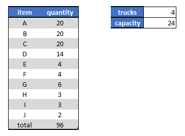
Given data:
try to load the trucks such that they have as few different items as possible. It is noted that our total truck capacity is exactly equal to the total quantity.

This looks like a simple, well-stated problem. We can minimize the maximum of the count of different items, or the sum. Here are a few solutions to illustrate this:


If we minimize the max count we can find the first or second solution: both have an optimal max count of 3. If we only focus on the sum, we can find the first or the last solution, both with a sum count of 11. The conclusion is: if we use min max count or min sum count as objective, we may see undesirable outcomes. So, if we want to develop a model that has a preference for solutions like the first one, we actually have to look at both, and use a multiple objective problem:

  1. Minimize the max count
  2. Minimize the sum count
(It is noted that here we have a case where there is a solution with optimal max count and optimal sum count. Often this is not the case: there may be trade-offs between the different objectives.)

A model using this approach can look like:


Weighted sum multi-objective model
\[\begin{align} \min \> & \color{DarkRed}{\mathit{MaxCount}} + \color{DarkBlue} w\cdot \color{DarkRed}{\mathit{SumCount}}\\ & \sum_j \color{DarkRed} x_{i,j} = \color{DarkBlue}{\mathit{Quantity}_i} & \forall i \\ & \sum_i \color{DarkRed} x_{i,j} \le \color{DarkBlue}{\mathit{Capacity}} & \forall j \\ & \color{DarkRed} x_{i,j} \le \min(\color{DarkBlue}{\mathit{Quantity}_i},\color{DarkBlue}{\mathit{Capacity}}) \cdot \color{DarkRed} y_{i,j} & \forall i,j \\ & \color{DarkRed}{\mathit{MaxCount}} \ge \sum_i \color{DarkRed} y_{i,j} & \forall j \\ & \color{DarkRed}{\mathit{SumCount}} = \sum_{i,j} \color{DarkRed} y_{i,j} \\ & \color{DarkRed} x_{i,j} \ge 0 \\ & \color{DarkRed} y_{i,j} \in \{0,1\} \end{align}\]

The scalar \(w>0\) indicates the trade-off between MaxCount and SumCount.

Special Case


If we want to first optimize for MaxCount and then for SumCount, we can choose a small value for \(w\), e.g. \(w=0.01\). An alternative approach for this case would be:

  1. Solve with objective: \(\min \mathit{MaxCount}\)
  2. Fix MaxCount to its optimal value
  3. Solve with objective: \(\min \mathit{SumCount}\)

Quadratic Objective


Interestingly, there is a single objective that is an alternative for our multi-objective model:


Quadratic model
\[\begin{align} \min \> & \sum_j \left( \sum_i \color{DarkRed} y_{i,j} \right)^2 \\ & \sum_j \color{DarkRed} x_{i,j} = \color{DarkBlue}{\mathit{Quantity}_i} & \forall i \\ & \sum_i \color{DarkRed} x_{i,j} \le \color{DarkBlue}{\mathit{Capacity}} & \forall j \\ & \color{DarkRed} x_{i,j} \le \min(\color{DarkBlue}{\mathit{Quantity}_i},\color{DarkBlue}{\mathit{Capacity}}) \cdot \color{DarkRed} y_{i,j} & \forall i,j \\ & \color{DarkRed} x_{i,j} \ge 0 \\ & \color{DarkRed} y_{i,j} \in \{0,1\} \end{align}\]

This objective will automatically put more emphasis on the larger column count values \( \sum_i y_{i,j} \) but still considers the small values. In essence, this is in-between a min max count and min sum count objective. In the picture with the solutions, you can see this objective denoted by sumsq count. This objective can properly distinguish between solution 1 and the other ones.

MIQP models are often more difficult to solve than linear MIP models. For large models, we often prefer the linear formulations.

Conclusion


Even what looks like a simple problem statement can have some wrinkles. It is not unusual that a problem ends up with a model with multiple objectives. This can guide the model to better behaved solutions essentially by using more complex incentives. 

References


Sunday, December 23, 2018

Linearizing multiple XOR operations

I have never encountered this in a model. but nevertheless this is an interesting question.

How can we handle \[y = x_1 \oplus x_2 \oplus \cdots \oplus x_n\] in a linear MIP model? Here \(\oplus\) indicates the xor operation. 

Well, when we look at \(x_1 \oplus x_2 \oplus \cdots \oplus x_n\) we can see that this is identical to \(\sum x_i\) being odd. A small example illustrates that:


Checking if an expression is odd can be done by seeing if it can not be expressed as \(2z\) where \(z\) is an integer variable. So combining this, we can do:

Linearization of \(y = x_1 \oplus x_2 \oplus \cdots \oplus x_n\)
\[\begin{align} & \color{DarkRed}y = \sum_i \color{DarkRed}x_i - 2 \color{DarkRed}z \\ & \color{DarkRed}y, \color{DarkRed} x_i \in\{0,1\} \\ & \color{DarkRed}z \in \{0,1,2,\dots\} \end{align}\]

If we want, we can relax \(y\) to be continuous between 0 and 1. An upper bound on z can be
\[z \le \left \lfloor{ \frac{n}{2} }\right \rfloor \].

References


  1. Express XOR with multiple inputs in zero-one integer linear programming (ILP), https://cs.stackexchange.com/questions/40737/express-xor-with-multiple-inputs-in-zero-one-integer-linear-programming-ilp
  2. XOR as linear inequalities, https://yetanothermathprogrammingconsultant.blogspot.com/2016/02/xor-as-linear-inequalities.html
  3. A variant of the Lights Out game, https://yetanothermathprogrammingconsultant.blogspot.com/2016/01/a-variant-of-lights-out-game.html

Friday, December 21, 2018

An interesting linearization involving xor

XOR gate sold by Amazon [1]


In [2] a question was asked:

How can we solve \[x^TAy = b\] for \(x_i, y_i \in \{-1,+1\}\)?

In this post I will discuss three different formulations:

  1. A simple quadratic formulation yielding a non-convex MIQCP model
  2. A MIP model based on a standard linearization
  3. A MIP model based on a linearization using an xor construct

Test Data


To help with some test models we need some data for \(A\) and \(b\). Here is an instance that actually has a solution (printed with 3 decimals):


----     13 PARAMETER a  

            i1          i2          i3          i4          i5

i1       0.998       0.579       0.991       0.762       0.131
i2       0.640       0.160       0.250       0.669       0.435
i3       0.360       0.351       0.131       0.150       0.589
i4       0.831       0.231       0.666       0.776       0.304
i5       0.110       0.502       0.160       0.872       0.265


----     13 PARAMETER b                    =        2.222 

Notice that solutions are not unique: if we have a solution \((x,y)\) then another solution is \((-x,-y)\).

MIQCP Model


The simplest is to use a Mixed-Integer Quadratically Constrained (MIQCP) model that handles the quadratic equation directly. Of course, in optimization we prefer binary variables \(z \in\{0,1\}\) instead of \(z \in\{-1,+1\}\). That is easily fixed: introduce binary variables \(p_i, q_i\) and write: \[\begin{align}&x_i = 2p_i-1\\&y_i = 2q_i-1\\&p_i,q_i \in\{0,1\}\end{align}\] This maps a binary variable to \(\{-1,+1\}\). So a MIQCP model can look like:

MIQCP Formulation
\[\begin{align} & \sum_{i,j} \color{DarkRed} x_i \color{DarkRed}y_j \color{DarkBlue}a_{i,j} = \color{DarkBlue}b \\ & \color{DarkRed}x_{i} = 2\color{DarkRed}p_{i}-1\\ & \color{DarkRed}y_{i} = 2\color{DarkRed}q_{i}-1\\ & \color{DarkRed}p_i, \color{DarkRed}q_i \in\{0,1\} \end{align}\]

This is a non-convex problem, so you need a global solver like Baron, Couenne or Antigone. Most quadratic solvers only support the much easier, convex case. When expressing this feasibility problem as an optimization problem, we need to add a dummy objective. The solution can look like:


----     55 VARIABLE p.L  

i1 1.000,    i4 1.000,    i5 1.000


----     55 VARIABLE q.L  

i1 1.000,    i2 1.000,    i4 1.000


----     55 VARIABLE x.L  

i1  1.000,    i2 -1.000,    i3 -1.000,    i4  1.000,    i5  1.000


----     55 VARIABLE y.L  

i1  1.000,    i2  1.000,    i3 -1.000,    i4  1.000,    i5 -1.000


----     59 PARAMETER b2                   =        2.222  x'Ay using solution values

We find a solution that when plugged into \(x^TAy\), reproduces our right-hand side.

Linearization 1


This problem can be linearized. This will allow us to use a linear MIP solver. One way is to write:\[\sum_{i,j} x_i y_j a_{i,j} = \sum_{i,j} (2p_i-1)(2q_j-1) a_{i,j} = \sum_{i,j} \left( 4 p_i q_j - 2 p_i -2q_j + 1 \right) a_{i,j} \]

The binary product \(v_{i,j} = p_i q_j\) can be linearized using a standard formulation [3]: \[\begin{align} &v_{i,j} \le p_i\\ &v_{i,j} \le q_j \\ & v_{i,j} \ge p_i + q_j -1 \\ & p_i, q_j, v_{i,j} \in \{0,1\} \end{align}\] Combining this leads to:

MIP Formulation I
\[\begin{align} & \sum_{i,j} \left( 4 \color{DarkRed} v_{i,j} - 2 \color{DarkRed}p_i -2 \color{DarkRed} q_j + 1 \right) \color{DarkBlue} a_{i,j} = \color{DarkBlue}b \\ & \color{DarkRed}v_{i,j} \le \color{DarkRed}p_i\\ & \color{DarkRed}v_{i,j} \le \color{DarkRed}q_j \\ & \color{DarkRed}v_{i,j} \ge \color{DarkRed}p_i + \color{DarkRed}q_j -1 \\ & \color{DarkRed}x_{i} = 2\color{DarkRed}p_{i}-1\\ & \color{DarkRed}y_{i} = 2\color{DarkRed}q_{i}-1\\ & \color{DarkRed}p_i, \color{DarkRed}q_i, \color{DarkRed}v_{i,j} \in\{0,1\} \end{align}\]

It is noted that \(v\) can be relaxed to be continuous between 0 and 1: \(v_{i,j} \in [0,1]\). The solution can look like:


----     62 VARIABLE p.L  

i1 1.000,    i4 1.000,    i5 1.000


----     62 VARIABLE q.L  

i1 1.000,    i2 1.000,    i4 1.000


----     62 VARIABLE v.L  v(i,j)=p(i)*q(j)

            i1          i2          i4

i1       1.000       1.000       1.000
i4       1.000       1.000       1.000
i5       1.000       1.000       1.000


----     62 VARIABLE x.L  

i1  1.000,    i2 -1.000,    i3 -1.000,    i4  1.000,    i5  1.000


----     62 VARIABLE y.L  

i1  1.000,    i2  1.000,    i3 -1.000,    i4  1.000,    i5 -1.000


----     66 PARAMETER b2                   =        2.222  x'Ay using solution values

Note that zeroes are not printed here (so the matrix \(v\) may look a bit strange).

Linearization 2


There is another linearization which is more interesting. For this we will use the binary xor operator.

There are different ways xor is denoted. I believe the most common ones are \[\begin{align} & z = x \textbf{ xor } y\\ & z = \textbf{xor}(x,y) \\ & z = x \oplus y \\ & z = x \veebar y\end{align}\] The xor truth table is: \[\begin{matrix} \textbf{ x } & \textbf{ y } & \textbf{ z }\\ 0 & 0 & 0 \\ 0 & 1 & 1 \\ 1 & 0 & 1\\ 1 & 1 & 0
\end{matrix}\]I.e. \(z = x \textbf{ xor } y \) is 1 if and only if \(x\) and \(y\) are different.

Now consider the following thruth-table:


----     15 PARAMETER t  truth-table

             x           y         x*y           p           q     p xor q   1 - 2 xor

i1          -1          -1           1                                               1
i2          -1           1          -1                       1           1          -1
i3           1          -1          -1           1                       1          -1
i4           1           1           1           1           1                       1

From this we can see that \[x_i  y_j = 1 - 2 (p_i \textbf{ xor } q_j) \] So our quadratic constraint becomes \[\sum_{i,j} x_i y_j a_{i,j} = \sum_{i,j} \left( 1 - 2 (p_i \textbf{ xor } q_j) \right)  a_{i,j} = b\] The operation \(w_{i,j} = p_i \textbf{ xor } q_j\)  can be linearized [4]: \[\begin{align} & w_{i,j} \le p_i + q_j \\& w_{i,j} \ge p_i - q_j \\& w_{i,j} \ge q_j - p_i \\& w_{i,j} \le 2 - p_i - q_j \\ & p_i, q_j, w_{i,j} \in \{0,1\} \end{align}\] With these tools we can formulate a different linearization:

MIP Formulation II
\[\begin{align} & \sum_{i,j} \left( 1 - 2 \color{DarkRed} w_{i,j} \right) \color{DarkBlue} a_{i,j} = \color{DarkBlue}b \\ & \color{DarkRed}w_{i,j} \le \color{DarkRed}p_i + \color{DarkRed}q_j\\ & \color{DarkRed}w_{i,j} \ge \color{DarkRed}p_i - \color{DarkRed}q_j \\ & \color{DarkRed}w_{i,j} \ge \color{DarkRed}q_j - \color{DarkRed}p_i \\ & \color{DarkRed}w_{i,j} \le 2 - \color{DarkRed}p_i - \color{DarkRed}q_j \\ & \color{DarkRed}x_{i} = 2\color{DarkRed}p_{i}-1\\ & \color{DarkRed}y_{i} = 2\color{DarkRed}q_{i}-1\\ & \color{DarkRed}p_i, \color{DarkRed}q_i, \color{DarkRed}w_{i,j} \in\{0,1\} \end{align}\]

It is noted that \(w\) can be relaxed to be continuous between 0 and 1: \(w_{i,j} \in [0,1]\). A solution can look like:

----     62 VARIABLE p.L  

i1 1.000,    i4 1.000,    i5 1.000


----     62 VARIABLE q.L  

i1 1.000,    i2 1.000,    i4 1.000


----     62 VARIABLE w.L  w(i,j) = p(i) xor q(j)

            i1          i2          i3          i4          i5

i1                               1.000                   1.000
i2       1.000       1.000                   1.000
i3       1.000       1.000                   1.000
i4                               1.000                   1.000
i5                               1.000                   1.000


----     62 VARIABLE x.L  

i1  1.000,    i2 -1.000,    i3 -1.000,    i4  1.000,    i5  1.000


----     62 VARIABLE y.L  

i1  1.000,    i2  1.000,    i3 -1.000,    i4  1.000,    i5 -1.000


----     66 PARAMETER b2                   =        2.222  x'Ay using solution values


Conclusion


I am somewhat surprised how different the two linearizations look. You would not easily recognize that the two different linear formulations are essentially the same. I don't remember many times I could use an xor operation in an optimization (I used it to solve Takuzu puzzles in [5]). The second linearization earns extra points for using xor!

This question was more interesting than I anticipated.

References


  1. A Fairchild/ON Semiconductor XOR gate sold by Amazon for $1.69. https://www.amazon.com/Logic-Gates-2-Input-XOR-Gate/dp/B00MEKUZV8
  2. Matrix Equation & Integer Programming, https://math.stackexchange.com/questions/3047086/matrix-equation-integer-programming/3047835
  3. Multiplication of Binary Variables, https://yetanothermathprogrammingconsultant.blogspot.com/2008/05/multiplication-of-binary-variables.html
  4. XOR as linear inequalities, https://yetanothermathprogrammingconsultant.blogspot.com/2016/02/xor-as-linear-inequalities.html
  5. Solving Takuzu puzzles as a MIP using xor, https://yetanothermathprogrammingconsultant.blogspot.com/2017/01/solving-takuzu-puzzles-as-mip-using-xor.html

Monday, December 10, 2018

More queens problems (2)

In [1], I discussed the Minimum Dominating Set of Queens Problem. Here is a variant:

Given an \(n \times n\) chess board, place \(n\) queens on the board such that the number of squares not under attack is maximized. 

For an \(n=8\) problem, the maximum number of non-dominated squares is 11. An example is:

11 white pawns are not under attack

We base the model on the one in [1]. First we define two sets of binary variables:

\[\begin{align} & x_{i,j} = \begin{cases} 1 & \text{if square \((i,j)\) is occupied by a queen}\\ 0 & \text{otherwise}\end{cases} \\ & y_{i,j} = \begin{cases} 1 & \text{if square \((i,j)\) is under attack} \\ 0 & \text{otherwise}\end{cases}\end{align}\]

The model can look like:


Maximum Non-Dominated Squares Problem
\[\begin{align}\max& \>\color{DarkRed}z=\sum_{i,j} \left(1-\color{DarkRed} y_{i,j}\right)\\ & \sum_{j'} \color{DarkRed}x_{i,j'} + \sum_{i'} \color{DarkRed}x_{i',j} + \sum_{i',j'|i'-j'=i-j} \color{DarkRed}x_{i',j'} +\sum_{i',j'|i'+j'=i+j} \color{DarkRed}x_{i',j'}-3 \color{DarkRed} x_{i,j} \ge \color{DarkBlue}M \cdot \color{DarkRed}y_{i,j} && \forall i,j \\  & \sum_{i,j}  \color{DarkRed} x_{i,j} = n \\& \color{DarkRed}x_{i,j},\color{DarkRed}y_{i,j}\in\{0,1\} \end{align}\]

The funny term \(-3x_{i,j}\) is to compensate for double counting occurrences of \(x_{i,j}\) in the previous terms [1]. We need to find a reasonable value for \(M\). An upper bound is \(M=n\). For \(n=8\), there are 48 different optimal solutions.

The problem \(n=9\) has one structural optimal solution (with 18 unattacked positions), and 3 variants by symmetry:


Is there a good way to find only structural solutions? One way is to use your own cuts as in [4], If we want to use the solution pool technology, we need to invent a constraint that forbids some symmetry (or have an objective that favors some of symmetric versions).

References


  1. More queens problems, https://yetanothermathprogrammingconsultant.blogspot.com/2018/12/more-queens-problems.html
  2. Bernard Lemaire, Pavel Vitushinkiy, Placing \(n\) non-dominating queens on the \(n\times n\) Chessboard, 2011, https://www.ffjm.org/upload/fichiers/N_NON_DOMINATING_QUEENS.pdf
  3. Maximum Queens Chess Problem, https://www.gams.com/latest/gamslib_ml/queens.103

Saturday, December 8, 2018

More queens problems

In [1] the famous \(n\)-queens problem was discussed: how many queens can we place on a chess-board such that non of them are attacked by others. Interestingly, we had some non-obvious problem with Cplex enumerating the different configurations (due to tolerance issues).

A different problem is the Minimum Dominating Set of Queens Problem:
Find the minimum number of queens needed such that they dominate each square.
Here dominate means: either a square is under attack by at least one queen, or it is occupied by a queen.

To develop a Mixed Integer Programming model, we introduce the familiar binary variables:

\[x_{i,j} = \begin{cases} 1 & \text{if square \((i,j)\) is occupied by a queen}\\ 0 & \text{otherwise}\end{cases}\]

A square \((i,j)\) is dominated if:

  1. \(x_{i,j}=1\): a queen is located here. This case will be covered by the following other cases, so we don't have to worry about this.
  2. There is a queen in row \(i\): \[\sum_{j'} x_{i,j'} \ge 1\]
  3. There is a queen in column \(j\):\[\sum_{i'} x_{i',j} \ge 1\]
  4. There is a queen in the same diagonal. The diagonal is described by \((i',j')\) such that \(i'-j'=i-j\). So we have: \[\sum_{i',j'|i'-j'=i-j} x_{i',j'}\ge 1\] If you prefer you can write this as \[\sum_{i'|1 \le i'-i+j \le n } x_{i',i'-i+j} \ge 1 \] 
  5. There is a queen in the same anti-diagonal. The anti-diagonal is described by \((i',j')\) such that \(i'+j'=i+j\). So we have: \[\sum_{i',j'|i'+j'=i+j} x_{i',j'}\ge 1\] This can also be written as \[\sum_{i'| 1 \le i+j-i' \le n} x_{i',i+j-i'} \ge 1\]


We can write these conditions in one big constraint. So we can write:

Minimum Dominating Set of Queens Problem
\[\begin{align}\min& \>\color{DarkRed}z=\sum_{i,j} \color{DarkRed} x_{i,j}\\ & \sum_{j'} \color{DarkRed}x_{i,j'} + \sum_{i'} \color{DarkRed}x_{i',j} + \sum_{i',j'|i'-j'=i-j} \color{DarkRed}x_{i',j'} +\sum_{i',j'|i'+j'=i+j} \color{DarkRed}x_{i',j'} \ge 1 && \forall i,j \\ & \color{DarkRed}x_{i,j}\in\{0,1\} \end{align}\]

For an \(8\times 8\) board, we need 5 queens. Here are two solutions:


You can verify that every unoccupied square is under attack.

Note that this formulation actually does a bit of double counting. E.g. when we look at the constraint for cell \((2,3)\) we see:


e(2,3)..  x(1,2) + x(1,3) + x(1,4) + x(2,1) + x(2,2) + 4*x(2,3) + x(2,4)
     
      + x(2,5) + x(2,6) + x(2,7) + x(2,8) + x(3,2) + x(3,3) + x(3,4) + x(4,1)
     
      + x(4,3) + x(4,5) + x(5,3) + x(5,6) + x(6,3) + x(6,7) + x(7,3) + x(7,8)
     
      + x(8,3) =G= 1 ; (LHS = 0, INFES = 1 ****)


We see that x(2,3) has a coefficient 4. This is harmless. However it looks a bit unpolished. With a little bit more careful modeling we can get rid of this coefficient 4. A complicated way would be: \[ \sum_{j'}x_{i,j'} + \sum_{i'|i'\ne i} x_{i',j} + \sum_{i',j'|i'-j'=i-j,i'\ne i, j'\ne j} x_{i',j'} +\sum_{i',j'|i'+j'=i+j,i'\ne i, j'\ne j} x_{i',j'} \ge 1 \>\> \forall i,j\] The first summation includes \(x_{i,j}\) while the other three summations exclude explicitly an occurrence of \(x_{i,j}\). Simpler is just to subtract \(3 x_{i,j}\): \[\sum_{j'} x_{i,j'} + \sum_{i'} x_{i',j} + \sum_{i',j'|i'-j'=i-j} x_{i',j'} +\sum_{i',j'|i'+j'=i+j} x_{i',j'}-3x_{i,j} \ge 1\>\> \forall i,j\] Here we just compensate for the double counting.

Now we see:


e(2,3)..  x(1,2) + x(1,3) + x(1,4) + x(2,1) + x(2,2) + x(2,3) + x(2,4) + x(2,5)
     
      + x(2,6) + x(2,7) + x(2,8) + x(3,2) + x(3,3) + x(3,4) + x(4,1) + x(4,3)
     
      + x(4,5) + x(5,3) + x(5,6) + x(6,3) + x(6,7) + x(7,3) + x(7,8) + x(8,3)

      =G= 1 ; (LHS = 0, INFES = 1 ****)


When we ask: how many different solution are there?, we use again the Cplex solution pool. And again, we have our tolerance problem:


pool.absgapNumber of solutions
02
0.54860

As the objective is integer valued, in some sense an absolute gap tolerance of 0.5 seems the safest. With this we find the correct number of solutions [2]. See [1] for a more in-depth discussion of this tolerance problem.

References


  1. Chess and solution pool, http://yetanothermathprogrammingconsultant.blogspot.com/2018/11/chess-and-solution-pool.html.
  2. Weisstein, Eric W.,  Queens Problem, http://mathworld.wolfram.com/QueensProblem.html
  3. Henning Fernau, minimum dominating set of queens: A trivial programming exercise?, Discrete Applied Mathematics, Volume 158, Issue 4, 28 February 2010, Pages 308-318. This is about programming instead of modeling. The issues are very different.
  4. Saad Alharbi and, Ibrahim Venkat, A Genetic Algorithm Based Approach for Solving the Minimum Dominating Set of Queens Problem, Hindawi Journal of Optimization, Volume 2017. I am not sure why a meta-heuristic is a good choice for solving this problem: you will not find proven optimal solutions.