Some Matrix Balancing Experiments

This is about the matrix balancing problem.

We have three sets of data:

• A matrix with with entries \(\color{darkblue}A^0_{i,j}\ge 0\). 
• Row- and column-totals \(\color{darkblue}r_i\) and  \(\color{darkblue}c_j\).

The \(\color{darkblue}A^0\) matrix is collected from different sources than the row- and column-totals. So the matrix elements don't sum up to our totals. The problem is finding a nearby matrix \(\color{darkred}A\), so the row and column totals are obeyed. In addition, we want to preserve the sparsity pattern of  \(\color{darkblue}A^0\): zeros should stay zero. And also: we don't want to introduce negative numbers (preserve the signs). More formally:

Matrix Balancing Problem
\[\begin{align}\min\>&{\bf{dist}}(\color{darkred}A,\color{darkblue}A^0)\\ & \sum_i \color{darkred}A_{i,j} = \color{darkblue}c_j && \forall j\\ & \sum_j \color{darkred}A_{i,j} = \color{darkblue}r_i && \forall i \\&\color{darkred}A_{i,j}=0 &&\forall i,j|\color{darkblue}A^0_{i,j}=0\\ &\color{darkred}A_{i,j}\ge 0 \end{align} \]

Approximate the matrix subject to row- and column-sum constraints

Data 

I invented some (random) data so we can scale the problem up to any size. The data generation algorithm is:

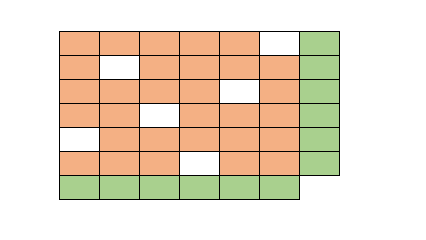
1. Generate the sparsity pattern of the matrix
2. Populate the non-zero elements of the matrix.
3. Calculate the row and column sums.
4. Perturb the row and column sums. I used a multiplication with a random number. This makes sure things stay positive.

Maintaining feasibility can be a bit finicky, especially if the matrix is sparse. Somehow it helps to perturb the totals instead of the matrix itself. 

I used a \(1000 \times 1000\) matrix in the experiments below.

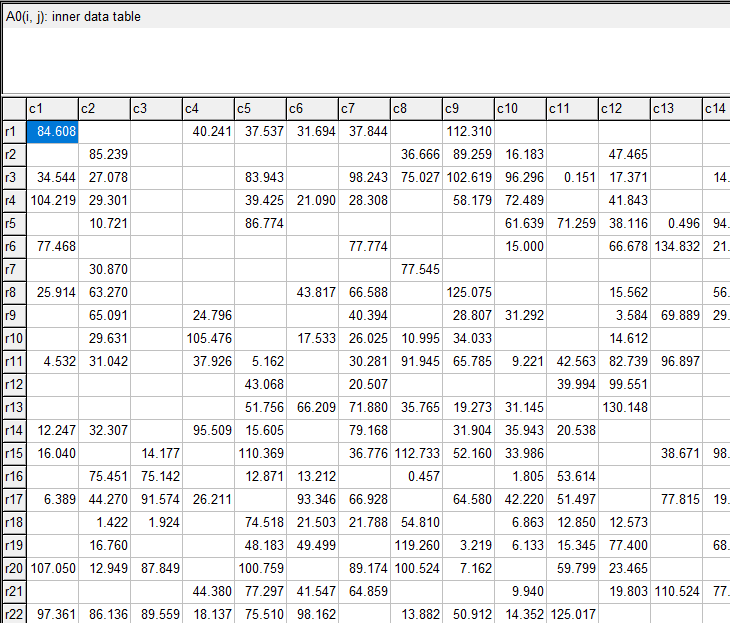Partial view of the generated matrix \(\color{darkblue}A^0\).

This is not a small problem, with about half a million (non-linear) variables. But this is still way smaller than the problems we may see in practice, especially when we regionalize.

The RAS algorithm

The RAS algorithm for bi-proportional fitting [1] is extremely popular. It is very simple, fast, and converges often in less than 10 iterations. The structure is as follows:

RAS Algorithm

\(\color{darkred}A_{i,j} := \color{darkblue}A^0_{i,j}\) loop   # row scaling   \(\color{darkred}\rho_i := \displaystyle\frac{\color{darkblue}r_i}{\sum_j \color{darkred}A_{i,j}}\)   \(\color{darkred}A_{i,j} := \color{darkred}\rho_i\cdot \color{darkred}A_{i,j}\)   # column scaling   \(\color{darkred}\sigma_j := \displaystyle\frac{\color{darkblue}c_j}{\sum_i \color{darkred}A_{i,j}}\)   \(\color{darkred}A_{i,j} := \color{darkred}\sigma_j\cdot \color{darkred}A_{i,j}\) until stopping criterion met

We can stop when an iteration limit is reached or when the quantities \(\rho_i\) and \(\sigma_j\) are sufficiently close to 1.0. In the GAMS code below, we stop either on iterations or on a converge measure.

Below I show the convergence speed by printing the maximum deviation from 1.0 for \(\rho_i\) and \(\sigma_j\). Or in different words: \[\left\|{{\rho-1}\atop{\sigma-1}}\right\|_{\infty}\] 

----     94 PARAMETER trace  RAS convergence

        ||rho-1||  ||sigm-1||    ||both||

iter1  0.04499855  0.05559031  0.05559031
iter2  0.00233051  0.00012370  0.00233051
iter3  0.00000958  0.00000059  0.00000958
iter4  0.00000004 3.587900E-9  0.00000004


----     95 RAS converged.
            PARAMETER niter                =        4.000  iteration number

This demonstrates excellent performance. Actually, it is quite phenomenal, when considering we are dealing with half a million non-linear variables \(\color{darkred}A_{i,j}\).

Entropy Maximization

The following Entropy based optimization model will give the same solutions as the RAS algorithm above.

The original entropy maximization problem has an objective of the form: \[\max\>H=-\sum_{i,j} b_{i,j} \ln b_{i,j}\] For our RAS emulation, we use a so-called cross entropy form: \[\min\>\sum_{i,j} b_{i,j} \ln \frac{b_{i,j}}{a_{i,j}}\] Our model becomes:

Cross-Entropy Optimization Problem
\[\begin{align}\min&\sum_{i,j|A^0_{i,j}\gt 0}\color{darkred}A_{i,j} \cdot \ln \frac{\color{darkred}A_{i,j}}{\color{darkblue}A^0_{i,j}}\\ & \sum_i \color{darkred}A_{i,j} = \color{darkblue}c_j && \forall j\\ & \sum_j \color{darkred}A_{i,j} = \color{darkblue}r_i && \forall i \\&\color{darkred}A_{i,j}=0 &&\forall i,j|\color{darkblue}A^0_{i,j}=0\\ &\color{darkred}A_{i,j}\ge 0 \end{align} \]

 

To protect the logarithm, I added a small lower bound on \(\color{darkred}A\): \(\color{darkred}A_{i,j} \ge \text{1e-5}\). 

Here are some results:

----    222 PARAMETER report  timings of different solvers

                obj        iter        time

RAS alg   -7720.083       4.000       0.909
CONOPT    -7720.083     124.000     618.656
IPOPT     -7720.083      15.000     171.602
IPOPTH    -7720.083      15.000      25.644
KNITRO    -7720.083      10.000      65.062
MOSEK     -7720.051      13.000      11.125

Notes:

• The objective in the RAS algorithm was just an evaluation of the objective function after RAS was finished.
• In the GAMS model, we skip all zero entries. We exploit sparsity.
• CONOPT is an active set algorithm and is not really very well suited for this kind of model. The model has a large number of super-basic variables. (Super-basic variables are non-linear variables between their bounds). CONOPT does better when a significant fraction of the non-linear variables are at their bound. In this model, all variables are non-linear and are between their bounds. 
• IPOPTH is the same as IPOPT but with a different linear algebra library (Harwell's MA27 instead of MUMPS). That has quite some impact on solution times.
• MOSEK is the fastest solver, but I needed to add an option: MSK_DPAR_INTPNT_CO_TOL_REL_GAP = 1.0e-5. This may need a bit more fine-tuning. Without this option, MOSEK would terminate with a message about a lack of progress. I assume it gets a little bit in numerical problems.
  
  The precise messages (without using this option) are:
  
  

  Interior-point solution summary
    Problem status  : UNKNOWN
    Solution status : UNKNOWN
    Primal.  obj: -7.7200665399e+03   nrm: 3e+04    Viol.  con: 3e-04    var: 0e+00    cones: 5e-05  
    Dual.    obj: -7.7200934976e+03   nrm: 1e+00    Viol.  con: 0e+00    var: 6e-10    cones: 0e+00  
  
  Return code - 10006 [MSK_RES_TRM_STALL]: The optimizer is terminated due to slow progress.
  

  
  
• MOSEK is not a general-purpose NLP solver. Older versions of MOSEK contained a general nonlinear convex solver, but this has been dropped. We have to use an exponential cone equation [4] for this entropy problem. This equation looks like: \[x_0 \ge x_1 \exp(x_2/x_1)\>\>\>\>\>\>\>\>x_0,x_1 \ge 0\]  To use this equation we need to reformulate things a bit. This is a little bit more work, requires a bit more thought, and the resulting model is not as natural or obvious as the other formulations.
• The difference between the CONOPT solution and RAS solution for \(\color{darkred}A\) is small: 
  ----    148 PARAMETER adiff                =  1.253979E-7  max difference between solutions
  This confirms we have arrived at the same solution. For the other solvers, I only compared the optimal objective function value.

Entropy Models [2]

References

1. Iterative Proportional Fitting, https://en.wikipedia.org/wiki/Iterative_proportional_fitting
2. Amos Golan. George Judge and Douglas Miller, Maximum Entropy Econometrics, Robust Estimation with Limited Data, Wiley, 1996
3. McDougall, Robert A., "Entropy Theory and RAS are Friends" (1999). GTAP Working Papers. Paper 6.
4. Dahl, J., Andersen, E.D., A primal-dual interior-point algorithm for nonsymmetric exponential-cone optimization. Math. Program. 194, 341–370 (2022).

Appendix: GAMS Model

$ontext    Matrix Balancing:    RAS vs Entropy Optimization $offtext *--------------------------------------------------------------- * size of the matrix *--------------------------------------------------------------- set    i 'rows' /r1*r1000/    j 'columns' /c1*c1000/ ; *--------------------------------------------------------------- * random sparse data *--------------------------------------------------------------- Set P(i,j) 'sparsity pattern'; P(i,j) = uniform(0,1)<0.5; Parameter A0(i,j) 'inner data table'; A0(p) = uniform(0,100); Parameter     r(i) 'known row sums'     c(j) 'known column sums' ; r(i) = sum(p(i,j), A0(p)); c(j) = sum(p(i,j), A0(p)); * * perturb A0 * A0(p) = uniform(0.5,1.5)*A0(p); *--------------------------------------------------------------- * RAS *--------------------------------------------------------------- set iter 'max RAS iterations' /iter1*iter50/; Scalars    tol    'tolerance' /1e-6/    niter  'iteration number'    diff1  'max(|rho-1|)'    diff2  'max(|sigma-1|)'    diff   'max(diff1,diff2)'    t      'time' ; parameters    A(i,j) 'updated matrix using RAS method'    rho(i) 'row scaling'    sigma(j) 'column scaling'    trace(iter,*) 'RAS convergence' ; t = timeElapsed; A(i,j) = A0(i,j); loop(iter,     niter = ord(iter); * * step 1 row scaling *    rho(i) = r(i)/sum(j,A(i,j));    A(i,j) = rho(i)*A(i,j); * * step 2 column scaling *    sigma(j) = c(j)/sum(i,A(i,j));    A(i,j) =  A(i,j)*sigma(j); * * converged? *    diff1 = smax(i,abs(rho(i)-1));    diff2 = smax(j,abs(sigma(j)-1));    diff = max(diff1,diff2);    trace(iter,'||rho-1||') = diff1;    trace(iter,'||sigm-1||') = diff2;    trace(iter,'||both||') = diff;    break$(diff < tol); ); option trace:8; display trace; if(diff < tol,   display "RAS converged.",niter; else   abort "RAS did not converge"; ); t = timeElapsed-t; parameter report 'timings of different solvers'; report('RAS alg','obj') = sum(p,A(p)*log(A(p)/A0(p))); report('RAS alg','iter') = niter; report('RAS alg','time') = t; display report; *--------------------------------------------------------------- * Entropy Model *--------------------------------------------------------------- variable z 'objective'; positive variable A2(i,j) 'updated table'; * initial point A2.l(p) = A0(p); * protect log A2.lo(p) = 1e-5; equations    objective  'cross-entropy objective'    rowsum(i)  'row totals'    colsum(j)  'column totals'    ; objective.. z =e= sum(p,A2(p)*log(A2(p)/A0(p))); rowsum(i).. sum(P(i,j), A2(p)) =e= r(i); colsum(j).. sum(P(i,j), A2(p)) =e= c(j); model m1 /all/; option threads=0, nlp=conopt; solve m1 minimizing z using nlp; *--------------------------------------------------------------- * Compare results * ||A2-A|| *--------------------------------------------------------------- scalar adiff 'max difference between solutions'; adiff = smax((i,j),abs(A2.l(i,j)-A(i,j))); display adiff; *--------------------------------------------------------------- * Try different solvers *--------------------------------------------------------------- report('CONOPT','obj') = z.l; report('CONOPT','iter') = m1.iterusd; report('CONOPT','time') = m1.resusd; A2.l(p) = 0; option nlp=ipopt; solve m1 minimizing z using nlp; report('IPOPT','obj') = z.l; report('IPOPT','iter') = m1.iterusd; report('IPOPT','time') = m1.resusd; A2.l(p) = 0; option nlp=ipopth; solve m1 minimizing z using nlp; report('IPOPTH','obj') = z.l; report('IPOPTH','iter') = m1.iterusd; report('IPOPTH','time') = m1.resusd; A2.l(p) = 0; option nlp=knitro; solve m1 minimizing z using nlp; report('KNITRO','obj') = z.l; report('KNITRO','iter') = m1.iterusd; report('KNITRO','time') = m1.resusd; display report; *--------------------------------------------------------------- * for mosek we use the exponential cone *--------------------------------------------------------------- positive variable x1(i,j); variable x3(i,j); a2.l(p) = 1; equations    expcone(i,j) 'exponential cone'    obj2         'updated objective'    defx1        'x1 = a0' ; obj2.. z =e= -sum(p,x3(p)); expcone(p).. x1(p) =g= a2(p)*exp(x3(p)/a2(p)); defx1(p).. x1(p) =e= a0(p); $onecho > mosek.opt MSK_DPAR_INTPNT_CO_TOL_REL_GAP = 1.0e-5 $offecho model m2 /obj2,expcone,rowsum,colsum,defx1/; option nlp=mosek; m2.optfile=1; solve m2 minimizing z using nlp; report('MOSEK','obj') = z.l; report('MOSEK','iter') = m2.iterusd; report('MOSEK','time') = m2.resusd; display report;