Portfolio Optimization: Maximize the Sharpe Ratio

The problem of finding the portfolio with the largest Sharpe Ratio can be written as: 

\[\boxed{\begin{align}\max\>&\frac{r^Tx-r_f}{\sqrt{x^TQx}}\\ & \sum_i x_i = 1\\ & x_i\ge 0\end{align}}\]

Of course we can add additional linear constraints \(Ax \sim b\):

\[\boxed{\begin{align}\max\>&\frac{r^Tx-r_f}{\sqrt{x^TQx}}\\ & \sum_i x_i = 1\\& Ax \sim b \\& x_i\ge 0\end{align}}\]

Here \(r_i\) are the returns, \(r_f\) is the risk-free return, and \(Q\) is the variance-covariance matrix. With \(\sim\) I indicate any relational operator \(\le,=,\ge\) This problem is not always trivial to solve. Here are some ideas.

1. Trace the Efficient Frontier

We can use the fact that the portfolio with the best Sharpe Ratio is located on the Efficient Frontier. When we plot the efficient frontier we solve the following model for different values of \(\lambda\ge 0\):

\[\boxed{\begin{align}\max\>&r^Tx-\lambda x^TQx\\&\sum_i x_i = 1\\ & Ax \sim b \\ & x_i\ge 0\end{align}}\]

Pick the point that has the best Sharpe Ratio.

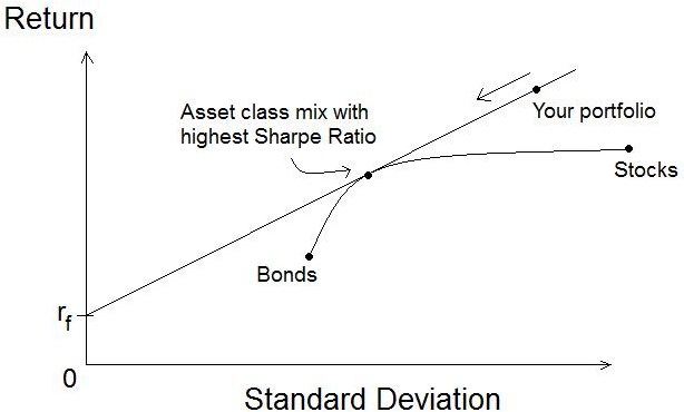
This picture (from here) shows the portfolio with the optimal Sharpe Ratio is located on the efficient frontier.

A more advanced method could be using a line search approach.

2. Use a general purpose  NLP solver

We can just throw the problem into an NLP solver. As long as the objective stays positive it is convex and we should be able to find the global optimum with a standard local NLP solver. When using a modeling system with automatic differentiation (such as AMPL and GAMS) it is quite easy to setup this model (no complicated gradients to worry about).

3. Use a QP solver

There is a somewhat non-trivial reformulation that allows us to solve this problem as a convex QP, provided that the return exceeds the rate-free return \(r_f\).  Note that we can check if a feasible portfolio exists with \(r^Tx-r_f>0\) by using a simple LP model. The transformed model has variables \(y\) and \(\kappa\) and looks like:

\[\boxed{\begin{align}\min\>&y^TQy\\ & \sum_i (r_i-r_f) y_i = 1\\ & \sum_i y_i = \kappa\\ & Ay \sim \kappa b \\ & y_i,\kappa \ge 0\end{align}}\]

We can retrieve the optimal value of \(x\) by \(x^*_i := y^*_i / \kappa^*\).

I usually prefer method (2) as the model resembles most closely the original intent. If you only have access to a quadratic solver, method (3) may be a good idea.

And finally, here is a picture of William (Bill) Sharpe:

(From here).

References

1. Gerard Cornuejols, Reha Tütüncü, Optimization Methods in Finance, Cambridge University Press, 2007
2. Leonid Kopman, Scott Liu, Maximizing the Sharpe Ratio and Information Ratio in the Barra Optimizer, MSCI Barra Research, 2009