Semi-continuous variables

A semi-continuous (or semicontinuous) variable $x$ is a continuous variable between bounds $[\ell,u]$ that also can assume the value zero. This is sometimes written as:

$$x \in \{0\} \cup [\ell,u]$$

I also see sometimes $x \in 0 \cup [\ell,u]$. I am not sure which version is more correct. We assume $0 \le \ell \le u$ (negative bounds are not very well defined in conjunction with semi-continuous variables).

Semi-continuous variables are often used in situations where we don’t like to see very small values. A standard example is a portfolio optimization problem where many small allocations are not very attractive (e.g. because of a transaction costs). Instead we prefer fewer instruments in the portfolio with larger allocations. This situation can be handled using semi-continuous variables.

There are a number of ways we can implement this. Some useful, some not so much.

$$\boxed{\begin{align}&\textbf{semi-continuous variable}\> x\\&x\in[\ell,u]\end{align}}$$	Many MIP solvers have a built-in type for semi-continuous variables. The values $\ell, u$ need to be specified as bounds on $x$. (Don’t specify them in equations, as in this case $x\ge\ell$ has a different meaning than $x^{lo}:=\ell$).
$$\boxed{\begin{align}&\ell\cdot \delta \le x \le u\cdot \delta\\&\delta \in \{0,1\}\\&x\in[0,u]\end{align}}$$	This is a standard way to model semi-continuous behavior using an extra binary variable $\delta$. In most cases the “sandwich” equation needs to be implemented as two separate constraints. The bounds on $x$ are not so relevant (e.g. we could have used a free variable).
$$\boxed{\begin{align}&x=\delta \cdot y\\&\delta\in \{0,1\}\\&y\in [\ell,u]\\&x\in [0,u]\end{align}}$$	A simple, intuitive non-linear (quadratic) formulation. Unfortunately many MIQP/MIQCP solvers will not accept this construct. We see many interesting and rather scary error messages. My favorite: Return code - 5010 [MSK_RES_ERR_MIO_INTERNAL]: A fatal error occurred in the mixed integer optimizer. Please contact MOSEK support. (May be you are asked to contact the Mosek people to apologize for doing this). The reason for all this havoc: a nonlinear equality constraint makes the model non-convex. In some cases we can replace $x=\delta\cdot y$ by an inequality to make things digestible for convex solvers.
$$\boxed{\begin{align}&x^2\ge \ell\cdot x\\&x\in [0,u]\end{align}}$$	Very compact and looks harmless. So nice try, but unfortunately also non-convex. There is just no way to create a convex formulation without the aid of some form of binary (or at least discrete) variables.

Every post should have preferably some graph, so here we go. This plots $x^2\ge \ell x$ for $\ell=10$.

References

• http://orinanobworld.blogspot.com/2011/03/semicontinuous-variables.html
• A strange issue with Cplex on a small model with semi-continuous variables: http://yetanothermathprogrammingconsultant.blogspot.com/2016/08/cplex-bug-or-not.html

Optimization in the news

https://techcrunch.com/2016/08/24/sigopt-series-a/

I don’t know this company, but it is good to see funding is available for optimization related endeavors. At first reading I suspected SigOpt was an ACM Special Interest Group, but that is not the case.

Back to basics: a very simple scheduling problem

In this post an extremely simple scheduling problem is proposed. But as we shall see, there are still a few interesting things to say about this. There are $n=9$ persons, two of which need to be available on-call each weekend. We need to design a schedule such that:

1. If a pair $(i,j)$ covers a weekend, then this same pair can not cover another weekend during the planning horizon. Persons $i$ and $j$ can form other pairs and in that configuration cover other weekends.
2. If a person $i$ covers a weekend $t$, he/she is off the next two weekends.

With $n=9$ persons we have $N=36$ possible pairs. The number is the same as the number of strictly sub-diagonal elements in a $n \times n$ matrix. This can be derived as $N=(n-1)+(n-2)+…+1+0 = \frac{1}{2}n(n-1)$. The number $N=36$ also dictates our planning window: if we have more than 36 weeks we need to recycle pairs.

Variables and equations

I propose to model this with two sets of binary variables:

• $x_{i,t} \in \{0,1\}$ is the assignment of person $i$ to duty on weekend $t$.
• $y_{i,j,t}\in \{0,1\}$ is the assignment of pair $(i,j)$ to weekend $t$. We say $(i,j)\in P$ to indicate we consider these unique $N=36$ pairs and not the full Carthesian product.

The rather obvious constraints on variable $y$ are:

$$\begin{align} & \sum_{(i,j)\in P} y_{i,j,t} = 1 & \forall t & \>\>\> \text{(1)} \\ & \sum_{t} y_{i,j,t} \le 1 & \forall (i,j) \in P & \>\>\>\text{(2)} \end{align}$$

Here equation (1) indicates we want exactly one pair per weekend and equation (2) implements no repeating occurrences of a pair $(i,j)$.

The constraint on variable $x$ is the implication: $x_{i,t}=1 \implies x_{i,t+1}=x_{i,t+2}=0$. Interestingly we can simply implement this as:

$$x_{i,t}+x_{i,t+1}+x_{i,t+2}\le 1\>\>\>\forall i,t\>\>\> \text{(3)}$$

The equivalence of these two restrictions may need a little bit of thought. It will prevent sequences like $[1,1]$ and $[1,0,1]$. We may need to pay a little bit of attention near the end of the planning period. In GAMS leads and lags that exceed the domain are automatically zero, and that is actually the correct behavior here. We end up with a last equation $x_{i,T}+0+0\le 1$ which we will assume the pre-solver of the MIP solver will remove. In AMPL you will need to handle the border conditions explicitly.

It is noted that equation (1) can also be written in terms of $x$. I.e. we could replace (1) by:

$$\sum_i x_{i,t} = 2\>\>\>\forall t \>\>\> \text{(1a)}$$

Finally we need connect $x$ and $y$. We can do this by $y_{i,j,t}=x_{i,t}\cdot x_{j,t}$. However this is non-linear. We can linearize this binary multiplication by:

$$\boxed{\begin{align}&y_{i,j,t}\le x_{i,t}\\ &y_{i,j,t}\le x_{j,t}\\&y_{i,j,t}\ge x_{i,t}+x_{j,t}-1 \end{align}}$$

$\forall (i,j)\in P, t$

$\>\>\text{(4)}$

If we use equation (1a) instead of (1) we can actually drop the first two inequalities of equation (4). This requires again a bit of thought. This step leaves $y$ floating in some cases. In essence we have relaxed the definition of $y$ somewhat: we use now $y_{i,j,t}\ge x_{i,t}\cdot x_{j,t}$. So when using this formulation, we should make sure to use only $x$ when reporting results. As noted in the comments, actually when using $T=36$, $y$ forms a proper schedule (Q: explain why) but when $T<36$ these floating $y$’s can be misleading as there may be spurious $y$’s being turned on. Hence, in this case only look at $x$ when reporting solutions. Of course if we want we can recover $y$ after the solve by evaluating $y^*_{i,j,t} := x^*_{i,t}\cdot x^*_{j,t}$.

There is no objective. As there is no objective the solver will stop at the first integer feasible point. This also means we do not need to worry about setting a gap tolerance optcr: the first integer feasible point found is immediately proven optimal. A constraint programming (CP) solver typically allow for a simpler representation of scheduling models, and I am pretty sure this will also be the case for this model.

Complete model and results

The complete model can look like:

A solution can look like:

Infinite horizon

In the model above we used a planning horizon of $N=36$ weeks. One way of dealing with longer horizons is to recycle the schedule: apply the schedule for week 1 to week 37. In this case we would have a violation of the two-weeks off rule:

Fixing this is not too complicated. We need to change equation (3) as follows:

$$\boxed{\begin{align}&x_{i,t}+x_{i,t+1}+x_{i,t+2}\le 1\>\>\>&\forall i,t<T-1\\&x_{i,T-1}+x_{i,T}+x_{i,1}\>\>\>&\forall i\\&x_{i,T}+x_{i,1}+x_{i,2}\>\>\>&\forall i \end{align}}$$

(3a)

where $T=36$ indicates the last week of the planning period.

In GAMS we can use the ++ operator for this and we can just write simply:

With this change the resulting schedule is:

Now we have a proper periodic schedule and we can recycle it starting in week 37. With this, we effectively have designed a steady state schedule that can be repeated ad infinitum. In other words, we have created a schedule with an infinite planning horizon.

Multi-objective optimization: an illustration

I saw some demonstrations of dynamic plots with the animation package in R.  So I was looking for a small example where I could try this out myself. So here we go.

In http://yetanothermathprogrammingconsultant.blogspot.com/2015/09/linearizations.html an example of a 2-objective land allocation problem is discussed. There are two competing objectives:

1. Minimize Cost: assign plots such that total development cost is minimal.
2. Maximize Compactness: cluster plots with the same land-use category together.

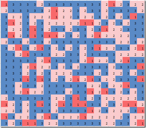
A pure cost based solution can look like the left picture below. When we take into account the compactness objective we could see something like the right picture.

Minimize Cost only	Minimize cost-α*compactness

These “plots” were just colored cells in an Excel spreadsheet. Now a more interesting and dynamic plot can be made if we play with the trade-off α between cost and compactness. That is done in the plot below. This was done using R and the packages ggplot2 and animation.

The bottom figure shows the efficient frontier. The curve indicates (cost,compactness) combinations that are Pareto optimal. This plot is in the f-space (the space of the objective functions). The top plot shows for different points along the efficient curve how the actual land assignment looks like. I.e. this plot is in the x-space: the space of the original decision variables. 

Notes

• If you pay careful attention you will notice that the dynamic plot and the static excel graphs have the y-axis reversed. In Excel row 1 starts at the top, while in R plots row 1 is at the bottom.
• It may be a good idea to apply some compactness constraints on political districts (in the US). This would reduce some of the crazy maps that are the result of gerrymandering. Compactness still can lead to unfair results, see: https://www.washingtonpost.com/news/wonk/wp/2015/03/01/this-is-the-best-explanation-of-gerrymandering-you-will-ever-see/.
• The above dynamic gif was the result of solving 50 MIP models.
• When generating HTML instead if a dynamic GIF VCR-style control buttons are added:
  

R Code

# # read results from GAMS model # setwd("c:/tmp/") library("RSQLite") sqlite <-dbDriver("SQLite") con <- dbConnect(sqlite, dbname="results.db") objs <- dbGetQuery(con,"select * from objs where objs in ('cost','compactness')") plotdata <- dbGetQuery(con,'select * from plotdata' ) dbDisconnect(con) library(ggplot2) library(gridExtra) library(animation) # # pivot df from long format to columns 'cost','compactness','a' # objs2 <- data.frame(cost=objs[objs$objs=="cost","value"], compactness=objs[objs$objs=="compactness","value"], id=objs[objs$objs=="cost","a"]) # needed to draw red lines indicating the current point on the curve mincost <- min(objs2$cost) maxcost <- max(objs2$cost) mincomp <- min(objs2$compactness) maxcomp <- max(objs2$compactness) N <- nrow(objs2) # # simple line plot of cost vs compactness # add lines to indicate where we are on the curve # plot2 <- function(currentCost,currentCompactness) { ggplot(data=objs2,aes(y=cost,x=compactness))+ geom_line(color="blue")+ annotate("segment", x = mincomp, xend = maxcomp, y = currentCost, yend = currentCost, color = "red")+ annotate("segment", x = currentCompactness, xend = currentCompactness, y = mincost, yend = maxcost, color = "red") } # # heatmap plot # plot1 <- function(pltdata) { pltdata$x <- as.integer(substr(pltdata$j,4,stop=100)) pltdata$y <- as.integer(substr(pltdata$i,4,stop=100)) pltdata$value <- as.factor(pltdata$value) ggplot(pltdata, aes(x=x, y=y, fill=value))+ geom_tile(color="black", size=0.1)+coord_equal()+ scale_fill_brewer(palette="Spectral",name="Land-use type")+ theme_classic()+ theme(axis.title.x=element_blank(), axis.text.x=element_blank(), axis.ticks.x=element_blank())+ theme(axis.title.y=element_blank(), axis.text.y=element_blank(), axis.ticks.y=element_blank())+ ggtitle("Land-use Optimization Results") } # # combine both plots # plot<-function(id) { pdata <- subset(plotdata,a==id) p1 <- plot1(pdata) cost <- objs2[objs2$id==id,"cost"] compactness <- objs2[objs2$id==id,"compactness"] p2 <- plot2(cost,compactness) grid.arrange(p1,p2,ncol=1,heights=c(1,0.5)) } # # animation # saveGIF({ for (i in 1:N) { # ids are of the form a1,a2,... id <- paste("a",i,sep="") print(plot(id)) if (i==1) { # add some pause print(plot(id)) print(plot(id)) } } },interval = 0.3, movie.name = "landuse.gif", ani.width = 600, ani.height = 800)

gdxrrw and R 3.3.1

From this post:

I have written a dispatch model in GAMS which optimizes by minimizing system costs. I want to loop runs of the model; Run the optimization, save the output, varying a single parameter(storageCap) -- increasing it by a small fraction each iteration, and running the model again. GDXRRW does not seem to be able to run on R v.3.3.1 -- "Bug In Your Hair".

Seems to work for me.

1. Install the R package gdxrrw:
   
   

   > install.packages("C:\\GAMS\\win64\\24.7\\gdxrrw\\win3264\\gdxrrw_1.0.0.zip",repos=NULL) Installing package into ‘C:/Users/Erwin/Documents/R/win-library/3.3’ (as ‘lib’ is unspecified) package ‘gdxrrw’ successfully unpacked and MD5 sums checked

   
   
2. Run a GAMS script like:
   
   

   set i /i1*i10/; parameter p(i); p(i) = uniform(0,1); display p; execute_unload "p.gdx",p; execute '"c:\program files\R\R-3.3.1\bin\Rscript.exe" p.R'; $onecho > p.R R.version library(gdxrrw) p<-rgdx.param("p.gdx","p"); p $offecho

I like to put external scripts at the bottom of the GAMS model in order to reduce the clutter. Background: as the $onecho is performed at compile time the script is actually written before we call it in the execute statement (which runs at execution time).

The output looks like:

--- Job Untitled_56.gms Start 08/18/16 15:29:58 24.6.1 r55820 WEX-WEI x86 64bit/MS Windows GAMS 24.6.1   Copyright (C) 1987-2016 GAMS Development. All rights reserved Licensee: Erwin Kalvelagen                               G150803/0001CV-GEN           Amsterdam Optimization Modeling Group                     DC10455 --- Starting compilation --- Untitled_56.gms(17) 3 Mb --- Starting execution: elapsed 0:00:00.013 --- Untitled_56.gms(5) 4 Mb --- GDX File C:\tmp\p.gdx --- Untitled_56.gms(6) 4 Mb                _                           platform       x86_64-w64-mingw32          arch           x86_64                      os             mingw32                     system         x86_64, mingw32             status                                     major          3                           minor          3.1                         year           2016                        month          06                          day            21                          svn rev        70800                       language       R                           version.string R version 3.3.1 (2016-06-21) nickname       Bug in Your Hair                 i          p 1   i1 0.17174713 2   i2 0.84326671 3   i3 0.55037536 4   i4 0.30113790 5   i5 0.29221212 6   i6 0.22405287 7   i7 0.34983050 8   i8 0.85627035 9   i9 0.06711372 10 i10 0.50021067 *** Status: Normal completion --- Job Untitled_56.gms Stop 08/18/16 15:29:59 elapsed 0:00:00.907

Portfolio Optimization: Maximize the Sharpe Ratio

The problem of finding the portfolio with the largest Sharpe Ratio can be written as: 

$$\boxed{\begin{align}\max\>&\frac{r^Tx-r_f}{\sqrt{x^TQx}}\\ & \sum_i x_i = 1\\ & x_i\ge 0\end{align}}$$

Of course we can add additional linear constraints $Ax \sim b$:

$$\boxed{\begin{align}\max\>&\frac{r^Tx-r_f}{\sqrt{x^TQx}}\\ & \sum_i x_i = 1\\& Ax \sim b \\& x_i\ge 0\end{align}}$$

Here $r_i$ are the returns, $r_f$ is the risk-free return, and $Q$ is the variance-covariance matrix. With $\sim$ I indicate any relational operator $\le,=,\ge$ This problem is not always trivial to solve. Here are some ideas.

1. Trace the Efficient Frontier

We can use the fact that the portfolio with the best Sharpe Ratio is located on the Efficient Frontier. When we plot the efficient frontier we solve the following model for different values of $\lambda\ge 0$:

$$\boxed{\begin{align}\max\>&r^Tx-\lambda x^TQx\\&\sum_i x_i = 1\\ & Ax \sim b \\ & x_i\ge 0\end{align}}$$

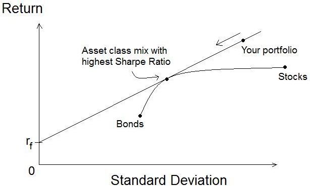
Pick the point that has the best Sharpe Ratio.

This picture (from here) shows the portfolio with the optimal Sharpe Ratio is located on the efficient frontier.

A more advanced method could be using a line search approach.

2. Use a general purpose  NLP solver

We can just throw the problem into an NLP solver. As long as the objective stays positive it is convex and we should be able to find the global optimum with a standard local NLP solver. When using a modeling system with automatic differentiation (such as AMPL and GAMS) it is quite easy to setup this model (no complicated gradients to worry about).

3. Use a QP solver

There is a somewhat non-trivial reformulation that allows us to solve this problem as a convex QP, provided that the return exceeds the rate-free return $r_f$.  Note that we can check if a feasible portfolio exists with $r^Tx-r_f>0$ by using a simple LP model. The transformed model has variables $y$ and $\kappa$ and looks like:

$$\boxed{\begin{align}\min\>&y^TQy\\ & \sum_i (r_i-r_f) y_i = 1\\ & \sum_i y_i = \kappa\\ & Ay \sim \kappa b \\ & y_i,\kappa \ge 0\end{align}}$$

We can retrieve the optimal value of $x$ by $x^*_i := y^*_i / \kappa^*$.

I usually prefer method (2) as the model resembles most closely the original intent. If you only have access to a quadratic solver, method (3) may be a good idea.

And finally, here is a picture of William (Bill) Sharpe:

(From here).

References

1. Gerard Cornuejols, Reha Tütüncü, Optimization Methods in Finance, Cambridge University Press, 2007
2. Leonid Kopman, Scott Liu, Maximizing the Sharpe Ratio and Information Ratio in the Barra Optimizer, MSCI Barra Research, 2009

10+ Free Open Source Solvers

http://www.butleranalytics.com/free-open-source-solvers/

I am pretty sure Gurobi and Mosek should not be in this list.

Update: Gurobi has been removed (now the list is exactly 10).

Wolfram Language

In http://blog.wolfram.com/2016/08/08/today-we-launch-version-11/ a new version of Mathematica is announced. More emphasis on the underlying language (Wolfram Language). I guess that makes sense: using the language as a unifying concept. Other interesting feature: 3D printing from Mathematica.

The tendency to attach Wolfram’s name to all products reminds me of a certain D. Trump. 

Simple Cutting Stock Example in R

In http://rpubs.com/KGFeMan/PM_IP an example of a cutting stock problem in solved in R using LpSolve. In this example all possible cutting patterns are generated in advance using some facilities of the iterpc package. A different way is to generate interesting patterns on the fly using a Column Generation scheme (see (1)).

References

1. Erwin Kalvelagen, Column Generation with GAMS, 2009,  http://www.amsterdamoptimization.com/pdf/colgen.pdf.

Cplex bug or not?

I was present at a GAMS demonstration yesterday, and I saw a strange thing. The model is a very small transportation model (model 1 in the GAMS model library):

$$\boxed{\begin{align}\min\>&\sum_{i,j} c_{i,j} x_{i,j}& \\ &\sum_j x_{i,j} \le a_i & \forall i \\ &\sum_i x_{i,j} \ge b_j & \forall j\\ &x_{i,j}\ge 0 \end{align}}$$

The twist is to make $x_{i,j}$ semi-continuous: $x_{i,j}=0$ or between $[100,1000]$. This can be modeled as:

$$\boxed{\begin{align} & 100 y_{i,j}\le x_{i,j} \le 1000 y_{i,j} \\ & y_{i,j} \in \{0,1\} \end{align}}$$

When looking at the log we saw:

Solution satisfies tolerances. MIP Solution:          159.525000    (3 iterations, 0 nodes) Final Solve:           156.375000    (0 iterations) Best possible:         153.675000 Absolute gap:            5.850000 Relative gap:            0.036671

I expect the highlighted numbers to be the same

Some background : by default GAMS solves a MIP with relative gap tolerance of 10%, so the MIP solution of  159.525 is not globally optimal but rather within 10% of the best possible solution. As GAMS wants to report marginals (duals and reduced costs) for a MIP, all integer variables are fixed and then the problem is resolved as an LP. This is the “Final Solve”. One would expect the same objective as the MIP solution, but here this is not the case. What is happening? Is this a bug?

Let’s compare the solutions.

MIP Solution (MIP solution found within gap tolerance) ----     78 VARIABLE y.L               new-york     chicago      topeka seattle         1.000 san-diego                   1.000       1.000 ----     78 VARIABLE x.L  shipment quantities in cases              new-york     chicago      topeka seattle       325.000 san-diego                 300.000     300.000 ----     78 VARIABLE z.L                   =      159.525  total transportation costs in thousands of dollars Final Solve (LP solution after fixing integer variables) ----     78 VARIABLE y.L               new-york     chicago      topeka seattle         1.000 san-diego                   1.000       1.000 ----     78 VARIABLE x.L  shipment quantities in cases              new-york     chicago      topeka seattle       325.000 san-diego                 300.000     275.000 ----     78 VARIABLE z.L                   =      156.375  total transportation costs in thousands of dollars

We see the discrete variables ($y$) are the same but one of the continuous variables ($x$) has changed.

Hypothesis: my guess is that the solution with $z=159.525$ was found using a heuristic instead of by solving this node using the standard dual simplex method. As a result this node may not be LP optimal. The log gives some hints:

Iteration      Dual Objective            In Variable           Out Variable      1  I            0.153000    x(seattle.new-york) demand(new-york) artif      2  I            0.000000     x(seattle.chicago)  demand(chicago) artif      3             153.675000  x(san-diego.new-york)  supply(seattle) slack Initializing dual steep norms . . . Iteration      Dual Objective            In Variable           Out Variable      1             153.675000e1(san-diego.new- slack  y(san-diego.new-york) Root relaxation solution time = 0.00 sec. (0.02 ticks)         Nodes                                         Cuts/    Node  Left     Objective  IInf  Best Integer    Best Bound    ItCnt     Gap *     0+    0                          159.5250       12.6000            92.10% Found incumbent of value 159.525000 after 0.11 sec. (0.11 ticks)         Nodes                                         Cuts/    Node  Left     Objective  IInf  Best Integer    Best Bound    ItCnt     Gap       0     0      153.6750     1      159.5250      153.6750        3    3.67%

Indeed it seems it took zero LP iterations to find the solution of 159.525 possibly by applying some heuristics on the root node solution. Somehow Cplex never solved that node to optimality after applying the heuristic, so we don’t see the 156.375 solution.

Now is this a bug? At first sight it is not. However an integer solution that is not LP optimal is actually often nonsensical. In the above example, the MIP solutions just ships too much to Topeka:

----     86 PARAMETER sol               new-york     chicago      topeka    capacity     shipped seattle       325.000                             350.000     325.000 san-diego                 300.000     300.000     600.000     600.000 demand        325.000     300.000     275.000 received      325.000     300.000     300.000

Obviously this solution does not pass the laugh test. I can see presenting such a solution to your boss may get you into trouble. As a result, I think reported MIP solutions should be LP optimal to prevent such meaningless solutions.

So this GAMS strategy of doing this final solve actually has a good side effect: cleaning up integer solutions. If you don’t use GAMS and use a gap tolerance: recheck your model solutions, because there may be issues with the continuous variables being non-optimal.

Note: this experiment was done with GAMS 24.7.3 and Cplex 12.6.3.0.

Conclusion: when using a gap tolerance Cplex can return solutions that are non-optimal with respect to the continuous variables. This is probably a bug. Although these solutions are (integer) feasible they can have undesirable characteristics. The way to repair these solutions is to fix the integer variables and resolve the model as an LP.

Dynamic programming vs MIP

Many problems solved by dynamic programming can also be formulated as a Mixed Integer Programming problem. Here is a very simple problem. The participant is asked to provide a Dynamic Programming algorithm that solves this problem to optimality. A MIP approach would be even simpler. Given $n$ gold mines located along a river. Each mine has a location $x_i$ (measured along the river) and has $w_i$ tons of gold. The goal is to select a subset of of the mines as pick-up points. The number of pick-up points is given: $k$. The cost to move gold from mine $i$ to pick-up point $j$ is $c_{i,j}=w_i |x_i-x_j|$.

This actually looks very much like an assignment problem:

$$\boxed{\begin{align} \min\>&\sum_{i,j} c_{i,j} x_{i,j}& \\ & \sum_j x_{i,j} = 1 &\forall i\\& \sum_i x_{i,j} = 1 &\forall j\\ & x_{i,j}\in \{0,1\} \end{align}}$$

We need to allow a destination $j$ to serve multiple sources $i$, so first we drop the second constraint. The second issue is that we need to count the number of destinations that are used. We can do this by introducing a binary variable $y_j$ with $\sum_j y_j=k$. If $y_j=0$ we need to ensure $x_{i,j}=0$. This can simply be modeled as $x_{i,j}\le y_j$. The complete model can now look like:

$$\boxed{\begin{align} \min\>&\sum_{i,j} c_{i,j} x_{i,j} & \\ & \sum_j x_{i,j} = 1 & \forall i\\& x_{i,j}\le y_j & \forall i,j\\ &\sum_j y_j = k \\& x_{i,j},y_j \in \{0,1\} \end{align}}$$

The solution for the example looks like

----     42 PARAMETER c  cost of moving i to j             mine1       mine2       mine3 mine1                  10.000      20.000 mine2      10.000                  10.000 mine3      20.000      10.000 ----     42 VARIABLE x.L  move i to j: assignment             mine2 mine1       1.000 mine2       1.000 mine3       1.000 ----     42 VARIABLE y.L  mine is collection point mine2 1.000

Notes:

1. We don’t need to worry about what happens with the gold already at a pick-up point. The model will automatically select $x_{j,j}=1$ when $j$ is a pick-up point as that is very cheap (i.e. $c_{j,j}=0$).
2. We can aggregate the equation $x_{i,j}\le y_j$ into $\sum_i x_{i,j} \le n \cdot y_j$. Often the disaggregated version shows better performance although we add more equations.
3. Without using a proper Dynamic Programming algorithm or a MIP/CP model this is more difficult. Here is an example of someone on the wrong track. Many programmers are not aware of these technologies.

Egyptian Vultures, Leaping Frogs and General Relativity

Some more exotic meta-heuristics with intriguing names:

See also: http://yetanothermathprogrammingconsultant.blogspot.com/2016/05/more-nature-inspired-heuristics.html

References

Thursday, August 25, 2016