> I don't understand the ordering of set elements
> in my display of a set.
If you look at:
set
i /a,c/
j /b,c/
;
display j;
then this will display:
---- 5 SET j
c, b
To understand this you'll need a little bit of knowledge how GAMS stores and orders set elements. Set elements are unique and stored in single large pool. They are ordered as they come. To display the pool (a.k.a universe) you can use:
alias (pool,*);
display pool;
This will show:
---- 8 SET pool Aliased with *
a, c, b
The ordering of elements (e.g. in display statements) is determined how they are ordered in the pool. It is also important in determining if a set is ordered (in that case the set follows the same ordering as the universe).
This can lead to surprises:
set
t1 /2001*2005/
t2 /2000*2006/;
display t2;
shows:
---- 5 SET t2
2001, 2002, 2003, 2004, 2005, 2000, 2006
A quick fix is to start with a dummy set to get the ordering correct:
set
dummy /2000*2010/
t1 /2001*2005/
t2 /2000*2006/;
display t2;
Wednesday, July 9, 2008


Monday, July 7, 2008
Bug in GAMS/Cplex link
GAMS/Cplex destroys here a perfectly good integer solution in the final LP. In that final LP the integers are fixed and the resulting LP is solved to get some dual information. In this case a resource limit is hit during this final LP and all is thrown away. Of course this is not what we want to see. The code in the GAMS/Cplex link related to this final LP solve need some careful inspection as we have seen problems with this part before.
A workaround is to increase reslim (so we have enough time to finish the final solve) or to decrease reslim (so we stop on time and allocate extra time to do the final solve). Note: as the duals are being used, it was no option to skip the final solve using option solvefinal.
Update: the GAMS people say the reported solution (primal+dual) should be ok.
I only have the log file, so I don't have evidence otherwise.
Repeating presolve.
Tried aggregator 2 times.
MIP Presolve eliminated 1679 rows and 1752 columns.
MIP Presolve modified 4 coefficients.
Aggregator did 23 substitutions.
Reduced MIP has 184571 rows, 180577 columns, and 758788 nonzeros.
Represolve time =    1.63 sec.
Clique table members: 37.
MIP emphasis: optimality.
MIP search method: dynamic search.
Parallel mode: opportunistic, using up to 4 threads.
Root relaxation solution time =  137.66 sec.

        Nodes                                         Cuts/
   Node  Left     Objective  IInf  Best Integer     Best Node    ItCnt     Gap

      0     0    14462.2442   195    14527.9285    14462.2442   178843    0.45%
Heuristic still looking.
Heuristic still looking.
*     0+    0                        14525.7851    14462.2442   178843    0.44%
      0     2    14462.2442   195    14525.7851    14462.2442   178843    0.44%
Elapsed real time = 4637.89 sec. (tree size =  0.00 MB, solutions = 8)
    100    99    14479.0518   197    14525.7851    14463.9712   232491    0.43%
                                                     Cuts: 15
    200   197    14490.7443   197    14525.7851    14463.9712   277649    0.43%
*   295+  286                        14525.5834    14463.9712   344217    0.42%
    300   295    14505.3123   147    14525.5834    14463.9712   336888    0.42%
    400   395    14514.1868   145    14525.5834    14463.9712   368746    0.42%
*   433+  408                        14525.5412    14463.9712   378611    0.42%
    500   476    14494.6548   134    14525.5412    14463.9712   420167    0.42%
                                                  Impl Bds: 1
*   544+  497                        14515.8473    14463.9712   437352    0.36%
*   545+  498                        14515.3114    14465.4987   441214    0.34%
Fixing integer variables, and solving final LP...
Tried aggregator 1 time.
LP Presolve eliminated 188052 rows and 205219 columns.
Aggregator did 6758 substitutions.
Reduced LP has 157128 rows, 152946 columns, and 633350 nonzeros.
Presolve time =    1.13 sec.
Initializing dual steep norms . . .

Iteration log . . .
Iteration:     1   Dual objective     =          6057.310401
Perturbation started.
Iteration:   102   Dual objective     =          6057.310401
Iteration:   878   Dual objective     =          7666.791470
Iteration:  1500   Dual objective     =          9296.038149
Iteration:  2211   Dual objective     =          9824.349977
Iteration:  2889   Dual objective     =         10466.849833
Iteration:  3542   Dual objective     =         10641.384471
Iteration:  4170   Dual objective     =         10892.599730
Iteration:  4795   Dual objective     =         10929.911432
Iteration:  5399   Dual objective     =         11011.407094
Iteration:  6008   Dual objective     =         11026.152235
Iteration:  6591   Dual objective     =         11028.613181
Iteration:  7181   Dual objective     =         11037.046345
Iteration:  7736   Dual objective     =         11039.881723
Iteration:  8318   Dual objective     =         11042.152553
Iteration:  8957   Dual objective     =         11044.445128
Iteration:  9519   Dual objective     =         11046.434903
Iteration: 10119   Dual objective     =         11048.475834
Iteration: 10685   Dual objective     =         11054.973343
Iteration: 11233   Dual objective     =         11057.071503
Iteration: 11774   Dual objective     =         11059.407174
Iteration: 12324   Dual objective     =         11062.135289
Iteration: 12869   Dual objective     =         11064.387325
Iteration: 13434   Dual objective     =         11066.637098
Iteration: 14031   Dual objective     =         11074.488101
Iteration: 14579   Dual objective     =         11076.981695
Iteration: 15089   Dual objective     =         11079.444173
Iteration: 15621   Dual objective     =         11082.365429
Iteration: 16145   Dual objective     =         11084.623184
Iteration: 16667   Dual objective     =         11087.253554
Iteration: 17199   Dual objective     =         11091.205312
Iteration: 17715   Dual objective     =         11098.091964
Iteration: 18262   Dual objective     =         11102.884193
Iteration: 18788   Dual objective     =         11106.328123
Iteration: 19295   Dual objective     =         11109.503749
Iteration: 19815   Dual objective     =         11114.531394
Iteration: 20324   Dual objective     =         11117.863392
Iteration: 20829   Dual objective     =         11120.704519
Iteration: 21333   Dual objective     =         11123.060983
Iteration: 21830   Dual objective     =         11128.551740
Iteration: 22365   Dual objective     =         11134.127949
Iteration: 22899   Dual objective     =         11137.954843
Iteration: 23365   Dual objective     =         11141.672390
Iteration: 23912   Dual objective     =         11149.342966
Iteration: 24419   Dual objective     =         11158.316182
Iteration: 24957   Dual objective     =         11179.374543
Iteration: 25473   Dual objective     =         11188.140937
Iteration: 26019   Dual objective     =         11193.656639
Iteration: 26520   Dual objective     =         11198.854075
Iteration: 27113   Dual objective     =         11209.155858
Iteration: 27664   Dual objective     =         11220.384286
Iteration: 28172   Dual objective     =         11228.944391
Iteration: 28665   Dual objective     =         11240.074822
Iteration: 29163   Dual objective     =         11246.180510
Iteration: 29682   Dual objective     =         11257.264795
Iteration: 30218   Dual objective     =         11275.780600
Iteration: 30745   Dual objective     =         11286.175702
Iteration: 31223   Dual objective     =         11293.826527
Iteration: 31706   Dual objective     =         11322.912597
Iteration: 32242   Dual objective     =         11345.656014
Iteration: 32792   Dual objective     =         11355.546099
Elapsed time =   10.16 sec. (33000 iterations).
Iteration: 33340   Dual objective     =         11365.028247
Iteration: 33859   Dual objective     =         11378.128137
Iteration: 34425   Dual objective     =         11384.719065
Iteration: 35106   Dual objective     =         11400.809173
Iteration: 35714   Dual objective     =         11410.512205
Iteration: 36277   Dual objective     =         11418.067340
Iteration: 36899   Dual objective     =         11440.861112
Iteration: 37511   Dual objective     =         11449.609068
Iteration: 38161   Dual objective     =         11461.996251
Iteration: 38848   Dual objective     =         11466.467047
Iteration: 39434   Dual objective     =         11479.910077
Iteration: 40002   Dual objective     =         11493.030687
Iteration: 40642   Dual objective     =         11500.724057
Iteration: 41217   Dual objective     =         11521.687737
Iteration: 41825   Dual objective     =         11532.637059
Iteration: 42526   Dual objective     =         11536.771010
Iteration: 43171   Dual objective     =         11541.448080
Iteration: 43797   Dual objective     =         11552.971322
Iteration: 44466   Dual objective     =         11565.311371
Iteration: 45131   Dual objective     =         11569.962544
Iteration: 45787   Dual objective     =         11574.606053
Iteration: 46461   Dual objective     =         11578.764831
Iteration: 47118   Dual objective     =         11588.017836
Iteration: 47736   Dual objective     =         11618.652276
Iteration: 48420   Dual objective     =         11627.910620
Iteration: 49100   Dual objective     =         11639.618577
Iteration: 49705   Dual objective     =         11709.154815
Iteration: 50257   Dual objective     =         11724.330084
Iteration: 50890   Dual objective     =         11731.428433
Iteration: 51600   Dual objective     =         11736.597227
Iteration: 52294   Dual objective     =         11744.978937
Iteration: 52895   Dual objective     =         11753.709220
Iteration: 53467   Dual objective     =         11765.418835
Iteration: 54163   Dual objective     =         11773.818329
Iteration: 54869   Dual objective     =         11780.943803
Iteration: 55550   Dual objective     =         11786.399499
Iteration: 56219   Dual objective     =         11792.327244
Iteration: 56894   Dual objective     =         11796.992322
Iteration: 57548   Dual objective     =         11800.527954
Iteration: 58177   Dual objective     =         11825.388844
Iteration: 58846   Dual objective     =         11838.119491
Iteration: 59544   Dual objective     =         11853.442610
Iteration: 60147   Dual objective     =         11864.848136
Iteration: 60781   Dual objective     =         11891.687076
Iteration: 61425   Dual objective     =         11906.740461
Iteration: 62087   Dual objective     =         11940.561093
Iteration: 62737   Dual objective     =         11975.219161
Elapsed time =   20.33 sec. (63000 iterations).
Iteration: 63454   Dual objective     =         12002.296415
Iteration: 64108   Dual objective     =         12015.440378
Iteration: 64818   Dual objective     =         12022.395479
Iteration: 65509   Dual objective     =         12029.058176
Iteration: 66219   Dual objective     =         12037.336718
Iteration: 66913   Dual objective     =         12048.634801
Iteration: 67550   Dual objective     =         12098.951656
Iteration: 68233   Dual objective     =         12148.667809
Iteration: 68861   Dual objective     =         12204.554100
Iteration: 69489   Dual objective     =         12260.068947
Iteration: 70151   Dual objective     =         12271.769079
Iteration: 71067   Dual objective     =         12340.904160
Iteration: 71916   Dual objective     =         12469.081691
Iteration: 72832   Dual objective     =         12538.397179
Iteration: 73689   Dual objective     =         12573.657042
Iteration: 74580   Dual objective     =         12633.804960
Iteration: 75466   Dual objective     =         12671.034083
Iteration: 76282   Dual objective     =         12709.759093
Iteration: 77157   Dual objective     =         12731.565162
Iteration: 78006   Dual objective     =         12791.001813
Iteration: 78861   Dual objective     =         12826.806885
Iteration: 79716   Dual objective     =         12862.410390
Iteration: 80579   Dual objective     =         12894.168594
Iteration: 81454   Dual objective     =         12987.178433
Iteration: 82296   Dual objective     =         13103.926493
Iteration: 83211   Dual objective     =         13321.544934
Iteration: 84091   Dual objective     =         13443.441166
Iteration: 84973   Dual objective     =         13562.343061
Iteration: 85890   Dual objective     =         13644.284360
Iteration: 86698   Dual objective     =         13720.220758
Iteration: 87401   Dual objective     =         13816.562168
Iteration: 88221   Dual objective     =         13881.829495
Iteration: 88849   Dual objective     =         13929.142875
Iteration: 89610   Dual objective     =         13984.379103
Iteration: 90422   Dual objective     =         14047.173914
Iteration: 91270   Dual objective     =         14115.140590
Iteration: 92125   Dual objective     =         14171.749778
Iteration: 93089   Dual objective     =         14217.148596
Iteration: 93982   Dual objective     =         14263.230690
Elapsed time =   30.39 sec. (94000 iterations).
Iteration: 94826   Dual objective     =         14320.598940
Iteration: 95556   Dual objective     =         14345.861439
Iteration: 96804   Dual objective     =         14379.439770
Iteration: 97540   Dual objective     =         14399.637101
Iteration: 98353   Dual objective     =         14415.843344
Iteration: 99135   Dual objective     =         14486.973327
Iteration: 100230   Dual objective     =         14507.696311
Iteration: 101753   Dual objective     =         14524.245965
Iteration: 102889   Dual objective     =         14536.589082
Iteration: 104245   Dual objective     =         14546.083262
Iteration: 105151   Dual objective     =         14553.547999
Iteration: 106121   Dual objective     =         14558.473735
Iteration: 107058   Dual objective     =         14562.528434
Iteration: 107846   Dual objective     =         14564.898252
Iteration: 108562   Dual objective     =         14568.707843
Iteration: 109171   Dual objective     =         14569.741540
Iteration: 110267   Dual objective     =         14570.230927
Iteration: 111442   Dual objective     =         14570.636373
Iteration: 113264   Dual objective     =         14570.833100
Iteration: 115164   Dual objective     =         14571.039823
Removing perturbation.
Iteration: 115366   Scaled dual infeas =             0.068957
Iteration: 118957   Scaled dual infeas =             0.000000
Iteration: 119095   Dual objective     =         14519.183719
Iteration: 119885   Dual objective     =         14526.787115
Elapsed time =   40.78 sec. (120000 iterations).
Iteration: 121024   Dual objective     =         14527.291310
Iteration: 121967   Dual objective     =         14527.804039
Iteration: 122614   Dual objective     =         14527.921795
Removing shift (76).
Iteration: 122721   Scaled dual infeas =             0.000158
Iteration: 122814   Dual objective     =         14527.911155
Removing shift (3).

Resource limit exceeded.

MIP Solution:        14527.928528    (0 iterations, 0 nodes)
Final Solve:         14527.928596    (122973 iterations)

Best possible:               -inf
Absolute gap:                  na
Relative gap:                  na
A workaround is to increase reslim (so we have enough time to finish the final solve) or to decrease reslim (so we stop on time and allocate extra time to do the final solve). Note: as the duals are being used, it was no option to skip the final solve using option solvefinal.
Update: the GAMS people say the reported solution (primal+dual) should be ok.
I only have the log file, so I don't have evidence otherwise.
Parallel processing of large models
> It might be desirable to invoke parallel processing of my optimization model
> on a network of PCs.
The simplest way to use parallel processing is to use a parallel solver such as Cplex, Xpress or Mosek and tell it to use multiple threads. E.g. with Cplex say threads 4 in an option file and it will exploit your quad core machine. Be aware that parallel processing is not always faster and that you need extra memory. This option only works on SMP machines (basically computers with multiple CPUs/cores).
If I remember correctly Xpress had once a version that worked on a network of machines using PVM. I don't think this was ever available under GAMS. GAMS/Xpress can use multiple threads, but again as SMP only.
GAMS has some grid facilities and the GAMS people have been pushing the Sun grid facility. In my experience this is all somewhat premature. The GAMS grid stuff is fragile and the Sun grid facility looks primitive. It would require quite some work to make this more user friendly. In addition, you need to make sure your model is suited for this type of architecture. The problem must be decomposable in a number of independent jobs, otherwise this approach won't work. Once you get this to work, in many cases you will find out that performance is often disappointing compared to a serial implementation on a fast PC.
Note that GAMS itself is single-threaded. I am not aware of a parallel modeling language although this would make sense for some classes of models. The block structure could be exploited for coarse-grained parallellism. The GAMS internals are very messy so I don't think this will be an option that will be added quickly.
> on a network of PCs.
The simplest way to use parallel processing is to use a parallel solver such as Cplex, Xpress or Mosek and tell it to use multiple threads. E.g. with Cplex say threads 4 in an option file and it will exploit your quad core machine. Be aware that parallel processing is not always faster and that you need extra memory. This option only works on SMP machines (basically computers with multiple CPUs/cores).
If I remember correctly Xpress had once a version that worked on a network of machines using PVM. I don't think this was ever available under GAMS. GAMS/Xpress can use multiple threads, but again as SMP only.
GAMS has some grid facilities and the GAMS people have been pushing the Sun grid facility. In my experience this is all somewhat premature. The GAMS grid stuff is fragile and the Sun grid facility looks primitive. It would require quite some work to make this more user friendly. In addition, you need to make sure your model is suited for this type of architecture. The problem must be decomposable in a number of independent jobs, otherwise this approach won't work. Once you get this to work, in many cases you will find out that performance is often disappointing compared to a serial implementation on a fast PC.
Note that GAMS itself is single-threaded. I am not aware of a parallel modeling language although this would make sense for some classes of models. The block structure could be exploited for coarse-grained parallellism. The GAMS internals are very messy so I don't think this will be an option that will be added quickly.
How to call GAMS from Access?
Short Answer: invoke gams.exe using the CreateProcess API call. In a practical application much more is needed:

- Create a button so user can launch GAMS
- Find the location where GAMS.EXE is located
- Create unique directory where scratch files can be read and written
- Provide a mechanism to write problem data to a GAMS file
- Call GAMS, capture log output and show in window, if needed add an interrupt button to stop the solution process
- Provide a mechanism to read solution data from the GAMS run
- Presentation of solution
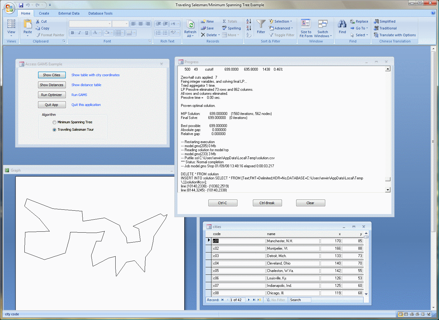
You'll see four windows inside Access. The first window contains some buttons that allow the user to drive the application. The log window shows any progress by GAMS. It also has some buttons to allow the user to interrupt the solution process. The graph is a simple way to display the solution. The right-lower window shows a data table with city related information (name, coordinates etc.)
Saturday, July 5, 2008
Bootstrap code for forming confidence intervals in Max Entropy estimation
Maximum entropy estimation has become an important tool when few observations are available. Some references are:
References:
- Amos Golan, George G. Judge, and Douglas Miller, Maximum Entropy Econometrics: Robust Estimation with Limited Data Wiley, 1996
- Channing Arndt, Sherman Robinson, and Finn Tarp, Parameter Estimation for a Computable General Equilibrium Model: A Maximum Entropy Approach http://www.ifpri.org/divs/tmd/dp/papers/tmdp40.pdf
- Erwin Kalvelagen, Least Squares Calculations with GAMS http://amsterdamoptimization.com/pdf/ols.pdf section 6
- Randall C. Campbell and R. Carter Hill, Maximum Entropy Estimation in Economic Models with Linear Inequality Restrictions, Tech. Report 2001-11, Louisiana State University, Department of Economics, 2001. http://ideas.repec.org/p/lsu/lsuwpp/2001-11.html
$ontext

   Bootstrap GME model

   Copyright 2007 Erwin Kalvelagen, Amsterdam Optimization

   References:
     [1] Maximum entropy estimation in economic models with linear
         inequality restrictions, Randall C. Campbell, R. Carter Hill
         Department of Economics, Louisiana State University,
         Baton Rouge, LA 70803,USA, 2001

     [2] Ramanathan, R., 2002. Introductory econometrics with applications
         (Harcourt College Publishers, Fort Worth).

     [3] Bardley Efron, Robert J. Tibshirani, "An Introduction to the Bootstrap",
         Chapman & Hall, 1993

   Files:
     bootstrap-gme.gms    -- gams file
     poverty.inc          -- data file
     tc.inc (optional)    -- file with quantiles for Student t distribution


$offtext


set i /case1*case116/
    k0 /
        constant 'constant term in regression'
        povrate  'poverty level'
        urb      'not used'
        famsize  'average household size'
        unemp    'percentage unemployment rate'
        highschl 'percentage of population age 25 and over with high school degree only'
        college  'percentage of population age 25 and over that completed 4 or more years of college'
        medinc   'median household income'
        D90      'dummy: one for the 1990 Census and zero for the 1980 Census'
      /
   k1(k0) 'data used' /povrate,famsize,unemp,highschl,college,medinc,D90/
;

*------------------------------------------------------------------------------
* input data from Ramanthan (2002, Data 7-6, p. 653)
*------------------------------------------------------------------------------

table data(i,k0) '-- input data from Ramanthan [2] (2002, Data 7-6, p. 653)'
$include poverty.inc
;
display data;


*------------------------------------------------------------------------------
* critical values t distribution
* this table is available from amsterdamoptimization.com
* if not available you can use a normal approximation
*------------------------------------------------------------------------------

$if exist tc.inc $include tc.inc
$if defined tc $goto tcok


* we have no access to tc.inc so we use a normal approximation

set prob /p1,p2,p3,p4,p5,p6/;
parameter probval(prob) /
  p1 0.10,  p2 0.05,  p3 0.025,  p4 0.01,  p5 0.005,  p6 0.001
/;

parameter qnorm(prob) /
  p1 1.281552, p2 1.644854, p3 1.959964, p4 2.326348, p5 2.575829, p6 3.090232
/;

$label tcok


*------------------------------------------------------------------------------
* create some summary statistics
*------------------------------------------------------------------------------

parameter summary(k1,*) '-- summary statistics (table 1 in [1])';
summary(k1,'mean') = sum(i,data(i,k1))/card(i);
summary(k1,'min') = smin(i,data(i,k1));
summary(k1,'max') = smax(i,data(i,k1));
summary(k1,'stdev') = sqrt[sum(i,sqr[data(i,k1)-summary(k1,'mean')])/(card(i)-1)];
summary(k1,'coeffvar') = summary(k1,'stdev')/summary(k1,'mean');
display summary;

*------------------------------------------------------------------------------
* linear regression using OLS
*------------------------------------------------------------------------------

set k(k0) 'regression coefficients'
    /constant,famsize,unemp,highschl,college,medinc,D90/;
data(i,'constant') = 1;

variables
  beta(k)  'regression coefficients'
  sse      'sum of squared errors'
;
equations
  dummyobj  'dummy objective'
  fit(i)    'fit linear equations'
;

dummyobj..   sse =n= 0;
fit(i)..     data(i,'povrate') =e=  sum(k, beta(k)*data(i,k));

model ols /dummyobj,fit/;

option lp=ls;
ols.limrow = 0;
ols.limcol = 0;
ols.solprint = 0;
solve ols using lp minimizing sse;

* Note: compare OLS results to page 8 in [1]

parameter estim(k,*,*) 'estimates';
estim(k,'OLS','-') = beta.l(k);

*------------------------------------------------------------------------------
* Calculate OLS confidence intervals
*------------------------------------------------------------------------------

parameter ols_se(k) 'standard errors';
ols_se(k) = beta.m(k);
display ols_se;

set ival 'confidence interval' /lo,up/;
scalar ndf 'degrees of freedom';
ndf = card(i) - card(k);
scalar alpha 'significance level' /0.025/;
scalar qt 'critical value';
$if defined tc        qt = sum((df,prob)$(dfval(df)=ndf and probval(prob)=0.025), tc(df,prob));
$if not defined tc    abort$(ndf<30) "Normal approximation not valid";
$if not defined tc    qt = sum(prob$(probval(prob)=0.025), qnorm(prob));
display ndf,alpha,qt;

parameter ols_conf_ival(k,ival);
ols_conf_ival(k,'lo') = beta.l(k) - qt*ols_se(k);
ols_conf_ival(k,'up') = beta.l(k) + qt*ols_se(k);
display ols_conf_ival;

* Note: these can also be imported from the GDX file LS.GDX
* See http://amsterdamoptimization.com/pdf/nlregression.pdf

*------------------------------------------------------------------------------
* GME model
*------------------------------------------------------------------------------

set j 'support points' /j1*j5/;

variables p(k,j), w(i,j);
p.lo(k,j) = 0.0001;
w.lo(i,j) = 0.0001;

variable
  entrpy      'entropy'
  e(i)        'residuals'
;
equations
  parmsupp(k) 'parameter support'
  errsupp(i)  'error support'
  normp(k)    'normalize p'
  normw(i)    'normalize w'
  obj         'maximize entropy'
  linear(i)   'linear model'
;

parameter
  z(k,j)      'parameter support matrix'
  v(i,j)      'error support matrix'
;

obj..          entrpy =e= -sum((k,j), p(k,j)*log(p(k,j)))-sum((i,j), w(i,j)*log(w(i,j)));
linear(i)..    data(i,'povrate') =e= sum(k, beta(k)*data(i,k)) + e(i);
parmsupp(k)..  beta(k) =e= sum(j, z(k,j)*p(k,j));
errsupp(i)..   e(i) =e= sum(j, v(i,j)*w(i,j));
normp(k)..     sum(j, p(k,j)) =e= 1;
normw(i)..     sum(j, w(i,j)) =e= 1;

model gme /obj,parmsupp,errsupp,linear,normp,normw/;


*------------------------------------------------------------------------------
* GME model support data
*------------------------------------------------------------------------------
set s 'error support scenarios' / s3, s4 /;
set gmex 'parameter support scenarios' /gme1,gme2,gme3/;

table z_all(gmex,k,j) 'parameter support for GME model'
                      j1   j2   j3   j4   j5
   gme1.constant     -50  -25    0   25   50
   gme1.famsize      -20  -10    0   10   20
   gme1.unemp        -20  -10    0   10   20
   gme1.highschl     -20  -10    0   10   20
   gme1.college      -20  -10    0   10   20
   gme1.medinc       -20  -10    0   10   20
   gme1.d90          -20  -10    0   10   20

   gme2.constant     -50  -25    0   25   50
   gme2.famsize      -10   -5    0    5   10
   gme2.unemp         -2   -1    0    1    2
   gme2.highschl      -2   -1    0    1    2
   gme2.college       -2   -1    0    1    2
   gme2.medinc       -10   -5    0    5   10
   gme2.d90          -20  -10    0   10   20

   gme3.constant     -50  -25    0   25   50
   gme3.famsize       -5    0    5   10   15
   gme3.unemp         -1    0    1    2    3
   gme3.highschl      -3   -2   -1    0    1
   gme3.college       -3   -2   -1    0    1
   gme3.medinc       -15  -10   -5    0    5
   gme3.d90          -20  -10    0   10   20

;

table esup_all(s,j) 'error support'
        j1    j2  j3    j4  j5
   s3  -10  -5.0   0   5.0  10
   s4  -13  -6.5   0   6.5  13
;

display "GME support data",z_all,esup_all;

*------------------------------------------------------------------------------
* run GME scenarios
*------------------------------------------------------------------------------

gme.limrow=0;
gme.limcol=0;
gme.solprint=2;
gme.solvelink=2;
loop((s,gmex),
  z(k,j) = z_all(gmex,k,j);
  v(i,j) = esup_all(s,j);
  solve gme maximizing entrpy using nlp;
  estim(k,s,gmex)=beta.l(k);
);

*------------------------------------------------------------------------------
* report results
*------------------------------------------------------------------------------

option estim:3:1:2;
display "---------------------------------------------------",
        "OLS and GME estimates (table 5 in [1])",
        "---------------------------------------------------",
         estim;

*------------------------------------------------------------------------------
* create bootstrap sample
*------------------------------------------------------------------------------


set nbs 'bootstrap samples' /sample1*sample400/;

parameter random(nbs,i) 'random draws with replacement';
random(nbs,i) = uniformint(1,card(i));
display random;

alias (i,ii);
set srandom(nbs,i,ii) 'as random but now expressed as a set';
srandom(nbs,i,ii)$(ord(ii)=random(nbs,i)) = yes;
display srandom;


*------------------------------------------------------------------------------
* run bootstrap method
*------------------------------------------------------------------------------


parameter newdata(i,k0);

equation linear2(i) 'linear model';

linear2(i)..    newdata(i,'povrate') =e= sum(k, beta(k)*newdata(i,k)) + e(i);

model gme2 /obj,parmsupp,errsupp,linear2,normp,normw/;

gme2.limrow=0;
gme2.limcol=0;
gme2.solprint=2;
gme2.solvelink=2;

parameter estim2(nbs,k,s,gmex) 'estimates';

loop(nbs,
    newdata(i,k0) = 0;
    newdata(i,k0) =  sum(srandom(nbs,i,ii), data(ii,k0));

    loop((s,gmex),
       z(k,j) = z_all(gmex,k,j);
       v(i,j) = esup_all(s,j);
       solve gme2 maximizing entrpy using nlp;
       estim2(nbs,k,s,gmex)=beta.l(k);
    );
);

display estim2;

*------------------------------------------------------------------------------
* calculate bootstrap confidence intervals
* percentile method
*------------------------------------------------------------------------------


* call rank first not from within a loop so declarations can happen
set idummy/a/;
parameters
   xdummy(idummy) /a 1/
   rdummy(idummy)
;
$libinclude rank xdummy idummy rdummy


parameter bconfival2(k,*,*,ival) 'confidence interval percentile method -- table 13 in [1]';
bconfival2(k,'OLS','-',ival) = ols_conf_ival(k,ival);

parameter
   bb(nbs)    'values to be sorted'
   pct(ival)  'percentiles'
   r(nbs)     'rank'
;
loop((k,s,gmex),
   bb(nbs) = estim2(nbs,k,s,gmex);
   pct('LO') = 2.5;
   pct('UP') = 97.5;
$libinclude rank bb nbs r pct
   bconfival2(k,s,gmex,ival) = pct(ival);
);

option bconfival2:3:1:3;
display bconfival2;
References:
- Thomas Rutherford, Paul van der Eijk, A GAMS Utility for Ranking One-Dimensional Numeric Data, http://www.mpsge.org/gdxrank/
- table with critical values: http://amsterdamoptimization.com/models/bootstrap/tc.inc
- example data set: http://amsterdamoptimization.com/models/bootstrap/poverty.inc
- Model file: http://amsterdamoptimization.com/models/bootstrap/bootstrap-gme.gms
Friday, July 4, 2008
ps2pdf
This online converter is handy if one needs to convert a postscript file to PDF:
http://www.ps2pdf.com/convert.htm.
http://www.ps2pdf.com/convert.htm.
Question about presolve
>Both AMPL and AIMMS have a built-in presolver that reduces
>the size of a model before it is passed on to the solver.
>Does GAMS have a presolver?
No. GAMS does not have a built-in presolver. It only has an option to remove fixed variables (model.holdfixed=1;). Solvers like GAMS/Cplex, GAMS/CONOPT have a built-in presolver inside the solver, but solvers like MINOS, SNOPT, SBB do not have this and they will need to work on the full size of the model. There are a number of advantages of having a presolver built into the modeling system: all solvers benefit even those without their own presolver, the modeling system can often provide better error messages and other feedback, and a smaller model to pass on to the solver may be cheaper (less I/O and other overhead).
>the size of a model before it is passed on to the solver.
>Does GAMS have a presolver?
No. GAMS does not have a built-in presolver. It only has an option to remove fixed variables (model.holdfixed=1;). Solvers like GAMS/Cplex, GAMS/CONOPT have a built-in presolver inside the solver, but solvers like MINOS, SNOPT, SBB do not have this and they will need to work on the full size of the model. There are a number of advantages of having a presolver built into the modeling system: all solvers benefit even those without their own presolver, the modeling system can often provide better error messages and other feedback, and a smaller model to pass on to the solver may be cheaper (less I/O and other overhead).
Critical values for the Student's t distribution
Confidence intervals for OLS regression models require to look up values for the Student's t distribution. The following GAMS include file will implement such a table in GAMS readable format.
Example:
Example output:
- table with critical values: http://amsterdamoptimization.com/php_uploads/Download/tc.inc
- example data set: http://amsterdamoptimization.com/php_uploads/Download/poverty.inc
Example:
set i /case1*case116/
    k0 /
        constant 'constant term in regression'
        povrate  'poverty level'
        urb      'not used'
        famsize  'average household size'
        unemp    'percentage unemployment rate'
        highschl 'percentage of population age 25 and over with high school degree only'
        college  'percentage of population age 25 and over that completed 4 or more years of college'
        medinc   'median household income'
        D90      'dummy: one for the 1990 Census and zero for the 1980 Census'
      /
   k1(k0) 'data used' /povrate,famsize,unemp,highschl,college,medinc,D90/
;

*------------------------------------------------------------------------------
* input data from Ramanthan (2002, Data 7-6, p. 653)
*------------------------------------------------------------------------------

table data(i,k0) '-- input data from Ramanthan (2002, Data 7-6, p. 653)'
$include poverty.inc
;
display data;


*------------------------------------------------------------------------------
* critical values t distribution
*------------------------------------------------------------------------------

$include tc.inc

*------------------------------------------------------------------------------
* create some summary statistics
*------------------------------------------------------------------------------

parameter summary(k1,*) '-- summary statistics';
summary(k1,'mean') = sum(i,data(i,k1))/card(i);
summary(k1,'min') = smin(i,data(i,k1));
summary(k1,'max') = smax(i,data(i,k1));
summary(k1,'stdev') = sqrt[sum(i,sqr[data(i,k1)-summary(k1,'mean')])/(card(i)-1)];
summary(k1,'coeffvar') = summary(k1,'stdev')/summary(k1,'mean');
display summary;

*------------------------------------------------------------------------------
* linear regression using OLS
*------------------------------------------------------------------------------

set k(k0) 'regression coefficients'
    /constant,famsize,unemp,highschl,college,medinc,D90/;
data(i,'constant') = 1;

variables
  beta(k)  'regression coefficients'
  sse      'sum of squared errors'
;
equations
  dummyobj  'dummy objective'
  fit(i)    'fit linear equations'
;

dummyobj..   sse =n= 0;
fit(i)..     data(i,'povrate') =e=  sum(k, beta(k)*data(i,k));

model ols /dummyobj,fit/;

option lp=ls;
solve ols using lp minimizing sse;

parameter ols_se(k) 'standard errors';
ols_se(k) = beta.m(k);

set ival 'confidence interval' /lo,up/;
scalar ndf 'degrees of freedom';
ndf = card(i) - card(k);
scalar alpha 'significance level' /0.025/;
scalar qt 'critical value';
qt = sum((df,prob)$(dfval(df)=ndf and probval(prob)=0.025), tc(df,prob));
display ndf,alpha,qt;

parameter ols_conf_ival(k,ival);
ols_conf_ival(k,'lo') = beta.l(k) - qt*ols_se(k);
ols_conf_ival(k,'up') = beta.l(k) + qt*ols_se(k);
display ols_se,ols_conf_ival;
Example output:
 =======================================================================
   Least Square Solver
   Erwin Kalvelagen, November 2004, October 2006
 =======================================================================

         Parameter      Estimate    Std. Error       t value      Pr(>|t|)
  beta('constant')   0.21659E+02   0.55303E+01   0.39164E+01   0.15708E-03 ***
   beta('famsize')   0.18042E+01   0.11617E+01   0.15531E+01   0.12329E+00
     beta('unemp')   0.76467E-01   0.59044E-01   0.12951E+01   0.19803E+00
  beta('highschl')  -0.20135E+00   0.39135E-01  -0.51450E+01   0.11914E-05 ***
   beta('college')   0.21313E-01   0.45803E-01   0.46532E+00   0.64263E+00
    beta('medinc')  -0.41557E+00   0.46677E-01  -0.89030E+01   0.13484E-13 ***
       beta('D90')   0.85045E+01   0.10434E+01   0.81508E+01   0.66416E-12 ***
      ---
      Signif. codes:  0 `***' 0.001 `**' 0.01 `*' 0.05 `.' 0.1 ` ' 1

 Estimation statistics:
 Cases: 116  Parameters: 7  Residual sum of squares:   0.32146E+03
 Residual standard error:   0.17173E+01   on  109 degrees of freedom
 Multiple R-squared:   0.74583E+00  Adjusted R-squared:   0.73183E+00
 F statistic:   0.53307E+02 on 6 and 109 DF, p-value:   0.00000E+00

 DLL version: _GAMS_GDX_237_2007-01-09
 GDX file: ls.gdx


----   1276 PARAMETER ndf                  =      109.000  degrees of freedom
            PARAMETER alpha                =        0.025  significance level
            PARAMETER qt                   =        1.982  critical value

----   1281 PARAMETER ols_se  standard errors

constant 5.530,    famsize  1.162,    unemp    0.059,    highschl 0.039,    college  0.046,    medinc   0.047
D90      1.043


----   1281 PARAMETER ols_conf_ival

                  lo          up

constant      10.698      32.619
famsize       -0.498       4.107
unemp         -0.041       0.193
highschl      -0.279      -0.124
college       -0.069       0.112
medinc        -0.508      -0.323
D90            6.436      10.572
Tuesday, July 1, 2008
Fortran question
I'm building and running LSSolver, but there are some problems interfacing the linking code in ls.f90 with the various Fortran sources (from TOMS and for the Student-t inverse, for example) on Linux.
Yes, for these older fortan codes you may need to add/real_size:64, -r8, /autodouble or something similar to the command line to set the default real size. I think all fortran compilers have a flag like that so you don't have to edit all declarations.
Here is a list for some compilers:
- Visual Fortran: /real_size:64
- Intel Fortran: -real-size 64 (linux) or /real-size:64 (windows)
- Lahey/Fujitsu Fortran: -dbl
- gfortran: -fdefault-real-8
- g95: -r8
- IBM XL Fortran: -qrealsize=8
- SUN Fortran: -xtypemap=real:64
Converting MathProg (and AMPL) models to GAMS
The tool glpk2gams can convert models written in MathProg (subset of AMPL) so we can quickly assess how GAMS solvers perform on such a model.
If the model only has a .mod file, you can just use a single argument:
If the model also has a .dat file, you need to give all three command line arguments:
It is generating scalar GAMS code, so this is not suited to convert models that have to be maintained in GAMS.
If the model only has a .mod file, you can just use a single argument:
D:\glpk\glpk2gams\Debug>glpk2gams.exe diet.mod
Glpk Model filename: diet.mod
Gams filename: diet.gms

Reading model section from diet.mod...
Reading data section from diet.mod...
99 lines were read
Generating nb...
Generating cost...
Model has been successfully generated

Rows : 10  Columns : 20  Nonzero elements : 179
Writing diet.gms

D:\glpk\glpk2gams\Debug>
If the model also has a .dat file, you need to give all three command line arguments:
L:\glpk>glpk2gams egypt2.mod egypt2.gms egypt2.dat
Glpk Model filename: egypt2.mod
Gams filename: egypt2.gms
Data filename: egypt2.dat

Reading model section from egypt2.mod...
egypt2.mod:264: warning: unexpected end of file; missing end statement inserted
264 lines were read
Reading data section from egypt2.dat...
egypt2.dat:276: warning: unexpected end of file; missing end statement inserted
276 lines were read
Generating Psi...
Generating mbd...
Generating mbdb...
Generating mb...
Generating cc...
Generating ap...
Generating al...
Generating ai...
Model has been successfully generated

Rows : 285  Columns : 351  Nonzero elements : 1336
Writing egypt2.gms

L:\glpk>
It is generating scalar GAMS code, so this is not suited to convert models that have to be maintained in GAMS.
Subscribe to:
Posts (Atom)