Generate all solutions that sum up to one

In a post, the following question was posed:

We can select unique values  \(\displaystyle\frac{1}{i}\) for \(i=1,\dots,n\). Find all combinations that add up to 1.

A complete enumeration scheme was slow even for \(n=10\). Can we use a MIP model for this or something related?

A single solution is easily found using the model:

Mathematical Model
\[ \begin{align} & \sum_{i=1}^n \frac{1}{i} \cdot \color{darkred}x_i = 1 \\ & \color{darkred}x_i \in \{0,1\} \end{align}\]

As MIP solvers use all kinds of tolerances, we can only increase \(n\) to some reasonable number (maybe 100, or 1000). After that, the coefficients \(1/i\) become likely too small. 

This model in itself is not so interesting, but the task of generating all feasible solutions makes it worth some attention.

There are basically three approaches for generating all feasible solutions:

• Use a Constraint Programming (CP) tool. Most CP solvers have built-in facilities to return more than just a single solution. However, they also typically work with integer data. Few CP solvers allow fractional data. Here, we have fractional data by design. Converting to an integer problem can be done by scaling the constraint.
• Use a no-good constraint.  Solve, add a constraint (cut) to the model that forbids the current solution, and repeat until things become infeasible.
• Some MIP solvers have what is called a solution pool which can enumerate solutions. These methods are often very fast.

We will experiment with two datasets:

• \(n=12\). This has three solutions.
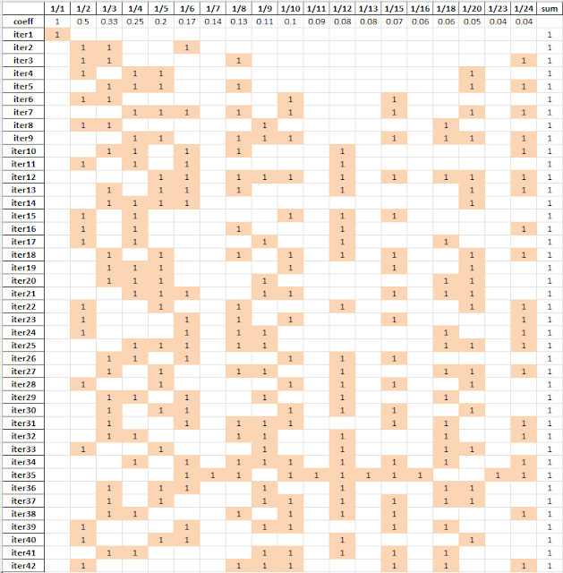
• \(n=25\). This gives us 41 solutions.

Constraint programming

Constraint programming solvers often work with discrete variables only. Furthermore, coefficients of the model are also often restricted to be integers. I am trying the small CP solver python-constraint [1]. From the documentation, it is not clear to me whether floating-point coefficients are allowed. When, I run the constraint as is, with coefficients \(1.0/i\), I see:

n=12
coefficients:[1.0, 0.5, 0.3333333333333333, 0.25, 0.2, 0.16666666666666666, 0.14285714285714285, 0.125, 0.1111111111111111, 0.1, 0.09090909090909091, 0.08333333333333333]
number of solutions: 2
['1/1']
['1/2', '1/3', '1/6']

This is not the correct answer.  These are certainly feasible solutions (the rows add up to one), but there is one more solution. So let's try to scale the constraint such that it has integer data. We can do this by writing: \[\sum_{i=1}^n \frac{\color{darkblue}{\mathit{LCM}}}{i} \cdot \color{darkred}x_i = \color{darkblue}{\mathit{LCM}}\] where \(\color{darkblue}{\mathit{LCM}}\) is the Least Common Multiple of \(\{1,\dots,n\}\). The coefficients \(\frac{\color{darkblue}{\mathit{LCM}}}{i}\) are now integers. When I solve it this way, I see:

n=12, lcm=27720
coefficients:[27720, 13860, 9240, 6930, 5544, 4620, 3960, 3465, 3080, 2772, 2520, 2310]
number of solutions: 3
['1/1']
['1/2', '1/3', '1/6']
['1/2', '1/4', '1/6', '1/12']

The coefficients are now integers. And we see all three solutions. The larger problem shows:

n=25, lcm=26771144400
number of solutions: 41
['1/1']
['1/2', '1/3', '1/6']
['1/2', '1/3', '1/8', '1/24']
['1/2', '1/3', '1/9', '1/18']
['1/2', '1/3', '1/10', '1/15']
['1/2', '1/4', '1/5', '1/20']
['1/2', '1/4', '1/6', '1/12']
['1/2', '1/4', '1/8', '1/12', '1/24']
['1/2', '1/4', '1/9', '1/12', '1/18']
['1/2', '1/4', '1/10', '1/12', '1/15']
['1/2', '1/5', '1/6', '1/12', '1/20']
['1/2', '1/5', '1/8', '1/12', '1/20', '1/24']
['1/2', '1/5', '1/9', '1/12', '1/18', '1/20']
['1/2', '1/5', '1/10', '1/12', '1/15', '1/20']
['1/2', '1/6', '1/8', '1/9', '1/18', '1/24']
['1/2', '1/6', '1/8', '1/10', '1/15', '1/24']
['1/2', '1/6', '1/9', '1/10', '1/15', '1/18']
['1/2', '1/8', '1/9', '1/10', '1/15', '1/18', '1/24']
['1/3', '1/4', '1/5', '1/6', '1/20']
['1/3', '1/4', '1/5', '1/8', '1/20', '1/24']
['1/3', '1/4', '1/5', '1/9', '1/18', '1/20']
['1/3', '1/4', '1/5', '1/10', '1/15', '1/20']
['1/3', '1/4', '1/6', '1/8', '1/12', '1/24']
...
['1/4', '1/5', '1/6', '1/9', '1/10', '1/15', '1/18', '1/20']
['1/4', '1/5', '1/8', '1/9', '1/10', '1/15', '1/18', '1/20', '1/24']
['1/4', '1/6', '1/8', '1/9', '1/10', '1/12', '1/15', '1/18', '1/24']
['1/5', '1/6', '1/8', '1/9', '1/10', '1/12', '1/15', '1/18', '1/20', '1/24']

The \(\color{darkblue}{\mathit{LCM}}\) is growing to a very large number. This second model took about 33 seconds. I believe this is using Python integer arithmetic (i.e., big ints), so this should be exact. I suspect that a solver like or-tools will have trouble with this, as it probably uses fixed-size integers. (The lcm number exceeds what fits in a 32-bit integer).

If a solver cannot handle floating-point coefficients, it really should refuse them with a proper message. I can understand why this solver does not like floating-point arithmetic: it requires that you need thinking this through and use appropriate tolerances. That makes things much more complicated.

No-good cuts

A no-good cut is a constraint that forbids a previously found integer solution, but nothing else. If we denote this integer solution by \(\color{darkblue}x^*_i\) then such constraint can look like: \[\sum_{i|\color{darkblue}x^*_i=1} \color{darkred}x_i - \sum_{i|\color{darkblue}x^*_i=0}\color{darkred}x_i \le \sum_{i|\color{darkblue}x^*_i=1}1 - 1 \] This can also be written as \[\sum_i (2 \color{darkblue}x^*_i -1)  \color{darkred}x_i \le \sum_i \color{darkblue}x^*_i - 1 \] The algorithm can look like:

1. Solve the model
2. If infeasible: STOP
3. Record the solution
4. Add the no-good cut to the model
5. Go to step 1

The output for the \(n=12\) case is:

----     75 PARAMETER trace  results for each iteration

              1/1         1/2         1/3         1/4         1/6        1/12         sum

coeff       1.000       0.500       0.333       0.250       0.167       0.083
iter1       1.000                                                                   1.000
iter2                   1.000       1.000                   1.000                   1.000
iter3                   1.000                   1.000       1.000       1.000       1.000

The larger problem with \(n=25\) has the following solution:

The solve loop for this problem took 11 seconds. We solved 43 MIP problems, i.e. 42 solutions (the last solve is infeasible). We have here one solution too many. This is likely a tolerance issue. We can tinker a bit with feasibility tolerances, something I loathe to do, but a model-based approach would be to form the following constraint: \[\sum_{i=1}^n \frac{1000}{i} \cdot \color{darkred}x_i = 1000 \]  This is a DIY scaling approach. This hopefully will prevent some very small coefficients (I am hedging here, as I don't know how the Cplex scaling algorithm interferes with this). Using this constraint, this algorithm generates 41 solutions. So, I am happy that this approach worked.

The corrected output looks like:

 

We basically dropped the iter35 solution from the previous picture, and as a result, some columns also got whacked.

Cplex solution pool

Again we used the scaled equation (with scale=1000).  With default settings, but with the constraint scaled by 1,000, I saw

--- Dumping 42 solutions from the solution pool...

This gives us one solution too many. (See [2] for a case where the Cplex solution pool also has problems.)  The fix is to tighten the integer feasibility tolerance a bit (I surrendered; as I really don't want to do that). Cplex allows me to set this to zero (unlike most other solvers), so that is what I did. The solution pool now returns the same set of solutions as the solve loop. The solution time is less than a second.

Conclusion

I used three methods to find all feasible integer solutions for this problem. There are a few small issues to resolve to make this work: 

• The constraint solver wants integer data, so I scaled the constraint by the LCM.
• The solve-loop with no-good constraints requires some attention. After scaling the constraint by 1000, I get the correct set of solutions
• The Cplex solution pool required me to change the integer feasibility tolerance.

For a small, almost trivial model, lots of little things go wrong. It is interesting that none of these approaches worked correctly just right out of the box. Solvers have become very powerful and are used more than ever before, but there is still lots of room for improvement.

References

1. Python-constraint, https://pypi.org/project/python-constraint/
2. Chess and Solution Pool, https://yetanothermathprogrammingconsultant.blogspot.com/2018/11/chess-and-solution-pool.html

Appendix: Python constraint code

import constraint as cp
import math 

n = 25
r = range(1,1+n)
lcm = math.lcm(*list(r))
print(f'n={n}, lcm={lcm}')

# coefficients 
p = [lcm // i for i in r] 
if n <= 15: print(f'coefficients:{p}')

problem = cp.Problem()
problem.addVariables(r, [0,1])
problem.addConstraint(cp.ExactSumConstraint(lcm,p))
sol = problem.getSolutions()
print(f'number of solutions: {len(sol)}')
for k in sol:
    print([f'1/{i}' for i in k.keys() if k[i]==1])

Appendix: GAMS model

$onText        Enumerate feasible solutions       1. using no-good constraints    2. using Cplex solution pool    $offText     *---------------------------------------------------------------- * data *----------------------------------------------------------------   set   dummy 'for ordering of elements' /'coeff'/   i 'numbers 1/i to use' /'1/1'*'1/25'/   k0 'iterations (superset)' /iter1*iter100/  ;   parameter p(i) 'coefficients'; p(i) = 1/ord(i);   *---------------------------------------------------------------- * dynamic set + parameters to hold cut data *----------------------------------------------------------------   set k(k0) 'iterations performed (and cut data index)'; k(k0) = no;   parameter cutcoeff(k0,*) 'coefficients for cuts'; cutcoeff(k0,i) = 0;   *---------------------------------------------------------------- * model * no-good cuts are added after each solve *----------------------------------------------------------------   binary variable x(i); variable z 'obj'; Equations   e     'sum to one'   cuts  'no-good cuts'   obj   'dummy objective' ;   scalar scale /1000/; e.. sum(i, scale*p(i)*x(i)) =e= scale; cuts(k).. sum(i,cutcoeff(k,i)*x(i)) =l= cutcoeff(k,'rhs'); obj.. z=e=0;   model m /all/; m.solprint = %solprint.Silent%; m.solvelink = %solveLink.Load Library%; option threads = 0;   *---------------------------------------------------------------- * algorithm *---------------------------------------------------------------- parameter trace(*,*) 'results for each iteration';   loop(k0,      solve m minimizing z using mip;      break$(m.modelstat <> 1 and m.modelstat <> 8);       x.l(i) = round(x.l(i));     trace(k0,i) = x.l(i);           cutcoeff(k0,i) = 2*x.l(i)-1;    cutcoeff(k0,'rhs') = sum(i,x.l(i))-1;    k(k0) = yes;        );     trace('coeff',i)$sum(k,trace(k,i)) = p(i); trace(k,'sum') = sum(i,p(i)*trace(k,i)); display trace;   *---------------------------------------------------------------- * solution pool approach *----------------------------------------------------------------   model m2 /obj,e/; m2.optfile=1; solve m2 minimizing z using mip;   $onecho > cplex.opt * solution pool options solnpoolintensity 4 solnpoolpop 2 populatelim 10000 solnpoolmerge solutions.gdx   * tighten tolerances epint 0 $offecho     * * load the gdx file with all solutions * set id /soln_m2_p1*soln_m2_p1000/; parameter xsol(id,i); execute_load "solutions.gdx",xsol=x; display xsol;