MIP Bounds

MIP (and related) solvers have a unique property: they provide a bound on the best possible integer solution at time \(t\). Together with the best-found integer solution so far, we have two bounds. Somewhere in between is the final optimal solution. The typical picture for these two bounds is as follows:

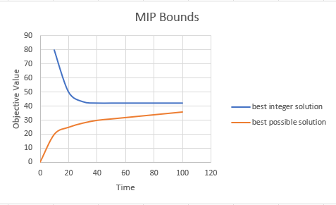
Typical shape

The vertical distance between the two curves is the gap. This is usually represented as a percentage. This picture is for minimization (maximization would turn things upside down). The overall idea is: in the beginning, we make much progress very quickly. Both the best integer solution found is improving a lot, and the best possible solution starts to converge very quickly. Then things start to get slower. Proving optimality takes more time. This form of the bounds tells us that it makes sense to stop early and accept the solution found so far (with a guaranteed quality measure).

We are extremely lucky the picture has the shape it has. Suppose it would look like:

This shape would be bad

This would mean: you really always have to run things to the end. Stopping early would give terrible solutions and terrible gaps. 

The two bounds are also known by different names. The best integer solution so far can be called incumbent, best-found or primal objective bound \(z_P\). The best possible solution is sometimes referred to as best-bound or dual objective bound \(z_D\).

Let's look at two actual examples. 

Example 1: crate picking

We have a collection of crates \(c\) that contain a different mix of products \(p\). Given a known demand for products \(p\), minimize the number of crates we need to use to satisfy this demand.

Model 1: minimize crate usage
\[\begin{align}\min& \sum_c \color{darkred}{\mathit{use}}_c\\ & \sum_c \color{darkblue}{\mathit{content}}_{c,p}\cdot\color{darkred}{\mathit{use}}_c \ge \color{darkblue}{\mathit{demand}}_p &&\forall p\\ & \color{darkred}{\mathit{use}}_c\in \{0,1\}\end{align}\]

The data set has 400 products and 4000 crates. The parameters \(\color{darkblue}{\mathit{content}}_{c,p}\) and \(\color{darkblue}{\mathit{demand}}_p\) are sparse: a crate doesn't contain every product, and there is demand for a subset of the products. The complete model is in an appendix.

The MIP objective bounds over time are as follows:

The red line is the objective value of the currently best integer solution, and the blue line is the objective value of the best possible solution. The height of the dark shaded area indicates the gap.

There are quite a few things we can see in this plot:

• The optimal solution was found quite early in the search, after about 140 seconds. Proving that this was the optimal solution took much longer: about another 1440 seconds. This is a great example where we can often interrupt the search much earlier and still find very good or even optimal solutions.
• The jump in the best bound near the end can be explained as follows. The objective has coefficients equal to one and binary variables. That means the objective changes by units of 1. So, if the best objective bound is less than 1 removed from the best-found solution, say 0.999, we can stop. We have proved optimality: there are no better solutions. Here the solver exploits a specific property of the objective function.
• Sometimes people ask how we can establish this best-bound. It is really based on math. We know with mathematical certainty that the search can not produce better solutions than the blue line. Some people suspect this probably has something to do with AI. No, just plain, old-fashioned math. 
• Near \(t=0\), some early relatively poor bounds are established but quickly tightened in the first few seconds or so. I ignore these in this plot to improve readability. For example, the objectives of the first few integer solutions were 3609, 3404, and 84. The best bound was initially zero. Plotting these would need a very tall y-axis, resulting in losing all details further down.
• For some data sets, this model is really difficult to solve to proven optimality. It makes sense to stop a bit earlier (or rather quite early) and accept the best solution found so far. It will be optimal or close to optimal.
• Sometimes the primal-dual integral (the size of the shaded area, between the best-possible and best-found integer solutions) is used to measure how well a MIP strategy performed. The MIP solver Xpress makes this quantity available. [1]
• All these measures are not scale-invariant. Although the "shape" of the curves is.

Example 2: evenly distribute items over bins

This model assigns items \(i\) to bins \(j\), in such a way that the variability between the sum of assigned values to bins is minimized. We do this by minimizing the maximum bin value. If we push down on the largest bin, eventually, things will even out.

Model 2: minimize variability
\[\begin{align}\min\>&\color{darkred}z\\ &\color{darkred}z \ge \sum_i  \color{darkblue}v_i \cdot \color{darkred}x_{i,j} && \forall j\\ & \sum_j \color{darkred}x_{i,j}=1 && \forall i \\ & \color{darkred}x_{i,j}\in \{0,1\}\end{align}\]

The data set has 500 items with random values \(\color{darkblue}v_i\) and 50 bins. The picture of the MIP bounds looks different:

 Notes:

• We see a ton of integer solutions. The best one was found after about 140 seconds (with an objective of 467.907). From that point on, until we hit the time limit of 3600 seconds, nothing happens. The gap is 0.11% after this best solution. This is guaranteed to be an excellent solution.
• The best bound is basically stuck at 467.407. From the beginning. 
• The x-axis has a square-root scale to see a bit better what is happening at the beginning.
• Again we can stop early.
• These models tend to be very difficult in terms of proving optimality.

References

1. https://www.fico.com/fico-xpress-optimization/docs/latest/solver/optimizer/HTML/PRIMALDUALINTEGRAL.html

Appendix 1: Model 1, crate picking

$ontext       Example 1       Minimize the number of crates to use     subject to demand for products is met.         Generate trace file for plotting   $offtext     *------------------------------------------------------------- * data *-------------------------------------------------------------   * * size of problem * set   p 'products' /prod1*prod400/   c 'crates' /crate1*crate4000/ ;   * * random sparse data * parameter    demand(p)    'demand for products'    content(c,p) 'content of crate' ;   demand(p)$(uniform(0,1)<0.1) = uniformint(1,100); content(c,p)$(uniform(0,1)<0.05) = uniformint(1,25);   *------------------------------------------------------------- * derived data *-------------------------------------------------------------   * * subset of interesting crates * set cu(c) 'crates with useful content'; * if no demand for any products in a crate, we'll ignore it. cu(c) = sum(p,content(c,p)*demand(p));   parameter crates(*) 'report on crates with useful content'; crates('total number of crates') = card(c); crates('useful crates') = card(cu); display crates;   * * feasibility check * parameter short(p) 'not enough products to meet demand'; short(p) = max(demand(p)-sum(c, content(c,p)),0); abort$sum(p,short(p)) 'can not meet demand',short;   *------------------------------------------------------------- * model *-------------------------------------------------------------   binary variable use(c) 'crate is used'; variable z 'objective';   equations    obj 'minimize number of crates to use'    meetdemand(p) 'demand must be met' ;    obj.. z =e= sum(cu(c), use(c)); meetdemand(p)$demand(p)..    sum(cu(c), content(c,p)*use(c)) =g= demand(p);   model m /all/; options threads=0, mip=cplex; m.optfile=1; solve m minimizing z using mip; *------------------------------------------------------------- * solver options *-------------------------------------------------------------   $onecho > cplex.opt miptrace trace1.csv $offecho

 

The code is doing a bit of presolving at the model level:

• Only generate the demand constraint when \(\color{darkblue}{\mathit{demand}}_p \gt 0\),
• Ignore crates that have no products we actually have demand for.

This is not really needed: the solver will take care of that in its presolver.

I prefer to write solver options at the end. This is a compile-time operation, so this is done before the solver optimizes the model.

This data set results in a model with 4,000 binary variables. This is not very small. Slight variations in the data can make the model much more difficult to solve to optimality. But we see near-optimal solutions very early in the search.

Appendix 2: Model 2, distributing items evenly

$onText       Example 2       Assign items to bins.     Minimize the maximum assigned values per bin.     This will give us an equal distribution of values     over the bins.         Generate trace file for plotting    $offText     *------------------------------------------------------------- * data *-------------------------------------------------------------   set   i 'items' /i1*i500/   j 'bins'  /bin1*bin50/ ;   parameter v(i) 'value'; v(i) = uniform(0,100); display v;   *------------------------------------------------------------- * model *-------------------------------------------------------------   binary variable x(i,j) 'assign items to bins'; variable z 'objective';   equations    itemOnce(i) 'place item once'    maxSum(j)   'max value in each bin' ;   itemOnce(i).. sum(j, x(i,j)) =e= 1; maxSum(j)..   z =g= sum(i, v(i)*x(i,j));   option threads=0, mip=cplex, reslim=3600; model m /all/; m.optfile=1; solve m minimizing z using mip;   *------------------------------------------------------------- * reporting *-------------------------------------------------------------   parameter sumval(j) 'values per bin'; sumval(j) = sum(i, v(i)*x.l(i,j)); display sumval,z.l; *------------------------------------------------------------- * solver options *------------------------------------------------------------- $onecho > cplex.opt miptrace trace2.csv $offecho

 

This model has 25,000 binary variables. That is quite large. It is not surprising it is very difficult to prove optimality. However, we find near-optimal solutions very early in the search.

There may be possibilities to handle symmetries better. One simple way would be to fix the first item to the first bin. A slightly more advanced method would restrict the \(i\)-th item to bins \(1,..,\min(i,|J|)\). (This worked for me: I could find slightly better solutions, resulting in a gap of 0.08%).  Another approach is to keep bins sorted by their value. 

An alternative objective would be to minimize the difference between the minimum and maximum bin values: \[\begin{align}\min\>&\color{darkred}u-\color{darkred}\ell \\ &\color{darkred}\ell \le \sum_i \color{darkblue}v_i \cdot \color{darkred}x_{i,j} \le \color{darkred}u && \forall j \\ &\sum_j \color{darkred}x_{i,j}=1 && \forall i \\ & \color{darkred}x_{i,j}\in \{0,1\} \end{align}\]

Unfortunately, this makes the problem not really much easier to solve.

Appendix 3: R script to plot trace

#--------------------------------------------------------------------------------
#
# plot MIP bounds from GAMS trace file
#
# GAMS/Cplex option: miptrace
#
#--------------------------------------------------------------------------------

#
# settings
#

filename <- "C:/Users/erwin/Downloads/trace2.csv"   # trace file 

title <- "MIP Model"                                # title of plot

xlo <- 3                                            # start of x-axis
ylo <- -1e10                                        # start of y-axis
yup <- 1e10                                         # end of y-axis

sqrt_axis <- T                                      # emphasize plot near t=0


#--------------------------------------------------------------------------------


library(tidyverse)


#
# read CSV file
#
hdr<-c("lineNum", "seriesID", "node", "seconds", "bestFound", "bestBound")
df<-read.csv(filename,na.strings = " na",header=F,comment.char="*",col.names=hdr)
  

#
# clip data
#
df$bestFound <- ifelse(df$bestFound>yup | df$bestFound<ylo | df$seconds < xlo, NA, df$bestFound)
df$bestBound <- ifelse(df$bestBound>yup | df$bestBound<ylo | df$seconds < xlo, NA, df$bestBound)
df$seconds <- ifelse(df$seconds<xlo,NA,df$seconds)

#
# Add column with found solutions
#
n <- nrow(df)
df$improvement[2:n] = diff(df$bestFound)
df$newSolution = ifelse(df$improvement != 0,df$bestFound,NA)


#
# convert to long format
#
df2 <- pivot_longer(df, c(bestFound,bestBound), names_to="bound", values_to="objective")

#
# plot of bounds
# 
p <- ggplot(data=df2,aes(x=seconds))+
  geom_line(aes(y=objective,color=bound),linewidth=0.7)+
  ggtitle(title)+theme(legend.position=c(.8, .9))+
  scale_color_manual(name="MIP Bounds",values=c("blue","red"),
                     labels=c("Best Possible Integer Solution",
                              "Best Found Integer Solution")) +
  geom_point(aes(y=newSolution)) + 
  geom_ribbon(data=df,aes(x=seconds,ymin=bestBound,ymax=bestFound),
              fill="grey",alpha=0.4) 
  if (sqrt_axis)  p <- p + scale_x_sqrt()  

print(p)

We start plotting after 3 seconds, so we don't include the extremely large initial bounds.