Yet Another Math Programming Consultant: Networks not always need an extra source and sink node

Convert standard assignment problem to a network problem

A standard assignment problem formulated as an LP/MIP looks like:

Assignment problem
\[\begin{align}\min&\sum_{i,j} \color{darkblue}c_{i,j}\cdot\color{darkred}x_{i,j}\\ & \sum_j \color{darkred}x_{i,j}=1 && \forall i \\ & \sum_i \color{darkred}x_{i,j}=1 && \forall j \\ & \color{darkred}x_{i,j} \in \{0,1\} \end{align}\]

The variables can be relaxed to be continuous between 0 and 1: solutions are integer-valued automatically. Let's denote the size of this problem as \(n = |I| = |J|\). This is a balanced assignment problem: the matrices \(\color{darkred}x_{i,j}\) and \(\color{darkblue}c_{i,j}\) are square.

On the OR-Tools website, a min-cost flow network problem is constructed that represents this assignment problem [1]. Here workers are to be assigned to tasks (or the other way around). The picture of the network is:

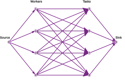Network from [1]

Let's summarize each type of node and arc in this network:

Node	Supply	Arc	Cost	Capacity
Source node	\(n\)	source\(\rightarrow\)worker	\(0\)	\(1\)
Worker nodes	\(0\)	worker\(\rightarrow\)task	\(c_{i,j}\)	\(1\)
Task nodes	\(0\)	task\(\rightarrow\)sink	\(0\)	\(1\)
Sink node	\(-n\)

Supply indicates inflow from outside (not from other nodes). A negative supply means we have a demand. In this formulation, source and sink are the only nodes with supply (and demand).

There is a more compact formulation: get rid of the source and the sink node. Something like:

So we have:

Node	Supply		Arc	Cost	Capacity
Worker nodes	\(1\)		worker\(\rightarrow\)task	\(c_{i,j}\)	\(1\)
Task nodes	\(-1\)

This makes the problem a little bit smaller. We save two nodes and \(2n\) arcs.

So why did they add the source and sink node? Maybe for aesthetic reasons: to isolate the supply to just the source and sink node? Or to be better prepared for unbalanced assignment problems (although the script needs modification to handle that)?

Of course, the savings in problem size are modest. So this is more a case of nitpicking on my side rather than a very serious issue.

The OR-tools library min-cost flow algorithm has a few quirks.

Only upper bounds (capacities) on the flows along the arcs are supported (lower bounds are always zero).
All coefficients are integers.
I believe there are no timing and iteration counts available (e.g. for comparison with an LP model —of course, iteration counts may be difficult to compare in any case).

An unbalanced variant

In [2], a different version of this problem is discussed. Here we have more tasks than workers. All tasks must be assigned (so workers may need to perform more than one task). In addition, we require that a worker need to perform at least one task.

As I think of the problem as assigning tasks to workers, let's use \(i\) to indicate tasks and use \(j\) for workers. The LP/MIP model can look like this:

Unbalanced assignment problem
\[\begin{align}\min&\sum_{i,j} \color{darkblue}c_{i,j}\cdot\color{darkred}x_{i,j}\\ & \sum_j \color{darkred}x_{i,j}=1 && \forall i \\ & \sum_i \color{darkred}x_{i,j}\ge 1 && \forall j \\ & \color{darkred}x_{i,j} \in \{0,1\}\end{align}\]

The matrices \(\color{darkred}x_{i,j}\) and \(\color{darkblue}c_{i,j}\) are no longer square. Again we can relax the \(\color{darkred}x_{i,j}\) variables to be continuous.

One way to view this as a network is:

We have \(n\gt m\), where \(n=|I|\) (number of tasks) and \(m=|J|\) (number of workers). The details of the network are

Node	Supply	Arc	Cost	Capacity
Task nodes	\(1\)	task\(\rightarrow\)worker	\(c_{i,j}\)	\(1\)
Worker nodes	\(-1\)	worker\(\rightarrow\)sink	\(0\)	\(n-m\)
Sink node	\(-(n-m)\)

The idea is to have a fixed demand of 1 (supply = -1) for the workers (this ensures we have at least one task for each worker). The remaining \(n-m\) tasks will end up in the sink.

If the algorithm allowed lower bounds on the flows, we could have a slightly different picture. We still would need outgoing arcs from the worker nodes. (They are needed to apply a lower bound on the flow.) But we wouldn't need the artificial demand. OR-tools' network code does not have lower bounds, so we use a negative supply on the worker nodes to force a flow of at least one.

Conclusion

A network model for a standard balanced assignment problem does not need a source and sink node. However, for some unbalanced problems, a source or sink can be useful.

Network algorithms often don't support lower bounds on flows (only upper bounds, a.k.a. capacities). In some cases, lower bounds can lead to more natural networks (closer to the original problem).

A network formulation is not always completely obvious. In addition, the code to generate the network is a bit further distanced from the original problem: reading the code does not immediately reveal the underlying problem. These are some of the reasons I usually implement these models as an LP. (Another reason is that LP/MIP models allow for richer problems, such as additional constraints.)

In this post, we used an explicit network representation. Another route is to formulate an LP model and tell the solver to solve it as a network, usually using a network Simplex method. The solver will extract the network from the LP model. This is supported by solvers like Cplex and Gurobi (the latest version). That will give you the opportunity to formulate a normal LP and still get the speed of a network solver. (But for large problems, this is slower than a hand-crafted network generator.)

References

Assignment as a Minimum Cost Flow Problem, https://developers.google.com/optimization/flow/assignment_min_cost_flow
Modified assignment problem (more tasks than agents), https://stackoverflow.com/questions/74606127/modified-assignment-problem-more-tasks-than-agents

Appendix: Python code for the balanced assignment problem

Adapted from [1]. This version drops the source and sink node (and the arcs involved).

#
# Revised implementation of linear assignment problem as network problem
#
from ortools.graph.python import min_cost_flow


# Instantiate a SimpleMinCostFlow solver.
smcf = min_cost_flow.SimpleMinCostFlow()

# Define the directed graph for the flow.
start_nodes = [0, 0, 0, 0, 1, 1, 1, 1, 2, 2, 2, 2, 3, 3, 3, 3] 
end_nodes   = [4, 4, 6, 7, 4, 5, 6, 7, 4, 5, 6, 7, 4, 5, 6, 7] 
capacities  = [1, 1, 1, 1, 1, 1, 1, 1, 1, 1, 1, 1, 1, 1, 1, 1]
costs       = [90, 76, 75, 70, 35, 85, 55, 65, 125, 95, 90, 105, 45, 110, 95, 115] 
supplies    = [1, 1, 1, 1, -1, -1, -1, -1]  
 
# Add each arc.
for i in range(len(start_nodes)):
    smcf.add_arc_with_capacity_and_unit_cost(start_nodes[i], end_nodes[i],
                                                 capacities[i], costs[i])
# Add node supplies.
for i in range(len(supplies)):
    smcf.set_node_supply(i, supplies[i])

# Find the minimum cost flow between supply and demand nodes .
status = smcf.solve()

if status == smcf.OPTIMAL:
    print('Total cost = ', smcf.optimal_cost())
    print()
    for arc in range(smcf.num_arcs()):
        # Arcs in the solution have a flow value of 1. Their start and end nodes
        # give an assignment of worker to task.
        if smcf.flow(arc) > 0:
            print('Worker %d assigned to task %d.  Cost = %d' %
                      (smcf.tail(arc), smcf.head(arc), smcf.unit_cost(arc)))
else:
    print('There was an issue with the min cost flow input.')
    print(f'Status: {status}')

Appendix: unbalanced assignment problem.

This code will solve the model: \[\begin{align}\min&\sum_{i,j} \color{darkblue}c_{i,j}\cdot\color{darkred}x_{i,j}\\ & \sum_j \color{darkred}x_{i,j}=1 && \forall i \\ & \sum_i \color{darkred}x_{i,j}\ge 1 && \forall j \\ & \color{darkred}x_{i,j} \in \{0,1\}\end{align}\] both as an LP and as a network model.

from ortools.linear_solver import pywraplp
from ortools.graph.python import min_cost_flow
import numpy as np

#
# sizes and (random) data
#
NTASK = 1000
NWORK = 200

# ORTOOLS min-cost flow wants integer costs
np.random.seed(123)
c = np.random.randint(1,100+1,(NTASK,NWORK))

#
# LP model
#
solver = pywraplp.Solver.CreateSolver('GLOP')

x = {(t,w):solver.NumVar(0.0, 1.0, f"x[t{t},w{w}]") for t in range(NTASK) for w in range(NWORK)}

solver.Minimize(sum([c[t,w]*x[(t,w)] for t in range(NTASK) for w in range(NWORK)]))

for t in range(NTASK):
    solver.Add(sum([x[(t,w)] for w in range(NWORK)]) == 1)
for w in range(NWORK):
    solver.Add(sum([x[(t,w)] for t in range(NTASK)]) >= 1)

#
# solve LP
#
status = solver.Solve()

if status == pywraplp.Solver.OPTIMAL:
    print(f'LP solver: Optimal objective value = {solver.Objective().Value()}')
    print(f'{solver.wall_time()/1000.0} seconds, {solver.iterations()} iterations')
else:
    print('LP solver: No optimal solution')
        
#
# network model
#
NNODES = NTASK + NWORK + 1
NARCS = NTASK*NWORK + NWORK

smcf = min_cost_flow.SimpleMinCostFlow()

# arcs
for t in range(NTASK):
    for w in range(NWORK):
        smcf.add_arc_with_capacity_and_unit_cost(t, NTASK+w, 1, c[t,w])                                                
for w in range(NWORK):
    smcf.add_arc_with_capacity_and_unit_cost(NTASK+w, NNODES-1, NTASK-NWORK, 0)
        
# nodes
for t in range(NTASK):
    smcf.set_node_supply(t, 1)
for w in range(NWORK):
    smcf.set_node_supply(NTASK+w, -1)
smcf.set_node_supply(NTASK+NWORK, -(NTASK-NWORK))    

# sanity check on bookkeeping
assert smcf.num_nodes() == NNODES       
assert smcf.num_arcs() == NARCS       

# solve
status = smcf.solve()
if status == smcf.Status.OPTIMAL:
    print(f"Network solver: Optimal objective value = {smcf.optimal_cost()}")  
else:
    print("Network solver: No optimal solution")

Yet Another Math Programming Consultant

Friday, December 2, 2022

Networks not always need an extra source and sink node