Micro-econometrics: discrete choice models

In this post, I want to discuss some statistical models from [1]. I'll implement these models in GAMS. First of all to emphasize these are all (nonlinear) optimization problems. Instead of using canned routines using a statistical package, this can help to get a better understanding of what is really going on. At least for me, not using a black-box routine, forces me to understand the underlying optimization models. Another application can be to have this part of a larger GAMS model. Some mathematical programming models just need some estimation code before the real model can be attacked. If the rest of the model is in GAMS, it may be a little bit easier to also use GAMS in the estimation tasks, instead of using a statistical package. This actually happens quite a lot. Finally, it may be easier to add constraints using a GAMS formulation compared to a canned routine in a statistical package.

In this case, the first argument was the reason for using GAMS. Reproducing results is for me a good tool to help me understand a dense text.  

Notation

When discussing statistical optimization models, it is always important to understand what is meant by \(x\) (or \(X\)). From a pure mathematical optimization point of view, \(x\) is often used to indicate decision variables. In statistics, \(X\) is often a data matrix. 

Similarly, the terms parameter and coefficient may mean different things in optimization and statistics. In mathematical programming parameters and coefficients are constants. For a regression, these terms indicate the quantities we want to estimate: they are decision variables in the mathematical optimization model.

This can cause some confusion.

Data

The problem we want to use in this experiment is from [2]: Does a new method of teaching economics (PSI) show improvements in grades (GRADE). The statistical variables (not optimization variables) are:

• GRADE: dependent variable indicating better grades in later economics classes,
• PSI: use of new teaching method (Personalized System of Instruction),
• GPA: Grade Point Average,
• TUCE: test score on the subject before entering the class

 

Data

OBS GPA TUCE PSI GRADE 1 2.66 20 0 0 2 2.89 22 0 0 3 3.28 24 0 0 4 2.92 12 0 0 5 4.00 21 0 1 6 2.86 17 0 0 7 2.76 17 0 0 8 2.87 21 0 0 9 3.03 25 0 0 10 3.92 29 0 1 11 2.63 20 0 0 12 3.32 23 0 0 13 3.57 23 0 0 14 3.26 25 0 1 15 3.53 26 0 0 16 2.74 19 0 0 17 2.75 25 0 0 18 2.83 19 0 0 19 3.12 23 1 0 20 3.16 25 1 1 21 2.06 22 1 0 22 3.62 28 1 1 23 2.89 14 1 0 24 3.51 26 1 0 25 3.54 24 1 1 26 2.83 27 1 1 27 3.39 17 1 1 28 2.67 24 1 0 29 3.65 21 1 1 30 4.00 23 1 1 31 3.10 21 1 0 32 2.39 19 1 1

Data Prep

To work with a more familiar notation, I create parameters \(y\) and \(X\). Also, a column with ones is added to \(X\), so we don't have to worry about adding a constant term to each of the models. So we form the following derived data:

----     79 PARAMETER y  dependent variable (grade)

case5  1.000,    case10 1.000,    case14 1.000,    case20 1.000,    case22 1.000,    case25 1.000,    case26 1.000
case27 1.000,    case29 1.000,    case30 1.000,    case32 1.000


----     79 PARAMETER X  independent variables

          constant         gpa        tuce         psi

case1        1.000       2.660      20.000
case2        1.000       2.890      22.000
case3        1.000       3.280      24.000
case4        1.000       2.920      12.000
case5        1.000       4.000      21.000
case6        1.000       2.860      17.000
case7        1.000       2.760      17.000
case8        1.000       2.870      21.000
case9        1.000       3.030      25.000
case10       1.000       3.920      29.000
case11       1.000       2.630      20.000
case12       1.000       3.320      23.000
case13       1.000       3.570      23.000
case14       1.000       3.260      25.000
case15       1.000       3.530      26.000
case16       1.000       2.740      19.000
case17       1.000       2.750      25.000
case18       1.000       2.830      19.000
case19       1.000       3.120      23.000       1.000
case20       1.000       3.160      25.000       1.000
case21       1.000       2.060      22.000       1.000
case22       1.000       3.620      28.000       1.000
case23       1.000       2.890      14.000       1.000
case24       1.000       3.510      26.000       1.000
case25       1.000       3.540      24.000       1.000
case26       1.000       2.830      27.000       1.000
case27       1.000       3.390      17.000       1.000
case28       1.000       2.670      24.000       1.000
case29       1.000       3.650      21.000       1.000
case30       1.000       4.000      23.000       1.000
case31       1.000       3.100      21.000       1.000
case32       1.000       2.390      19.000       1.000

The dependent variable grade is binary. To analyze models with this property, techniques like logit and probit are used. The independent variable psi is also binary. That is not changing much in the analysis.

  

Exercise

In this post, I want to reproduce some of the numbers from table 17.1 in [1]:

In this table APE stands for Average Partial Effects defined as: \[APE=\frac{1}{n}\sum_{i=1}^{n} f(\pmb{x}_i'\hat{\pmb{\beta}})\hat{\pmb{\beta}}\] For a discrete explanatory variable (PSI in our case), a different formula is used: \[APE=\frac{1}{n}\sum_{i=1}^{n} \left[ F(\pmb{x1}_i'\hat{\pmb{\beta}})-F(\pmb{x0}_i'\hat{\pmb{\beta}})\right]\] where \(\pmb{x1}_i\) is the i-th observation with \(PSI=1\) imputed, and similar,  \(\pmb{x0}_i\) is the i-th observation with \(PSI=0\) imputed. I did not completely understand the notation used in the footnote of table 17.1 for quite a while. Here I tried to use a different notation with some additional verbal explanation. In case of doubt, the precise implementation of this formula is in the GAMS model in the appendix.

Note that \(f(x)\) indicates the density and \(F(x)\) the cumulative distribution function. 

OLS: Ordinary Least Squares

Almost always, before looking into more complex models, it is a good idea to perform some standard linear regressions. I'll discuss a few ways of doing a least-squares fit. This is a bit of a side track, but I know that this is quite useful for many users. Least-squares is an important modeling concept.

The first optimization model is how I usually formulate least squares models in GAMS:

QP Model 1
\[\begin{align}\min&\sum_i \color{darkred}e_i^2 \\& \color{darkblue}y_i = \sum_j \color{darkblue}X_{i,j} \color{darkred}\beta_j + \color{darkred}e_i &&\forall i \end{align}\]

These are easy models, and they can be solved with any QP or NLP solver. We can substitute out \(\color{darkred}e_i\), and a more standard unconstrained QP follows:

Unconstrained QP Model 2
\[\min\>\sum_i \left(\color{darkblue}y_i - \sum_j \color{darkblue}X_{i,j} \color{darkred}\beta_j\right)^2 \]

This model is also often written in matrix notation: \[\min\>\|\color{darkblue}y-\color{darkblue}X\color{darkred}\beta\|_2^2\]

A method based on solving the so-called normal equations is as follows:

OLS Normal Equations
\[(\color{darkblue}X'\color{darkblue}X)\color{darkred}\beta = \color{darkblue}X'\color{darkblue}y\]

In GAMS, systems of equations can be solved as CNS (Constrained Nonlinear System) or MCP (Mixed Complementarity Problem) or using an LP/NLP with a dummy objective. Note that this method is numerically not very stable: when forming \((\color{darkblue}X'\color{darkblue}X)\) some very large numbers may be created.

A final approach can be to use some regression subroutine. These don't do any optimization, but typically use QR or SVD decomposition. For instance Python has several least squares functions (e.g., numpy.linalg.lstsq, sklearn.linear_model.LinearRegression, statsmodels.regression.linear_model.OLS). GAMS has an interface to the numpy.linalg.lstsq function. I believe this is using a divide-and-conquer SVD algorithm.

This last approach is recommended for numerically more challenging cases. For well-behaved problems, all methods should work. If there are constraints on the coefficients, the optimization models are obvious choices. 

For our data set, we see:

 

----    356 PARAMETER results  results from estimation methods

            OLS(QP1)    OLS(QP2)   OLS(NRML)     OLS(py)
               coeff       coeff       coeff       coeff

constant      -1.498      -1.498      -1.498      -1.498
gpa            0.464       0.464       0.464       0.464
tuce           0.010       0.010       0.010       0.010
psi            0.379       0.379       0.379       0.379

The interpretation is that we basically ignore that the dependent variable grade is a binary response. We just consider it as a standard, continuous response variable. The signs of the coefficients for gpa, tuce and psi make sense.

The APE (Average Partial Effect) for OLS is not so interesting. 

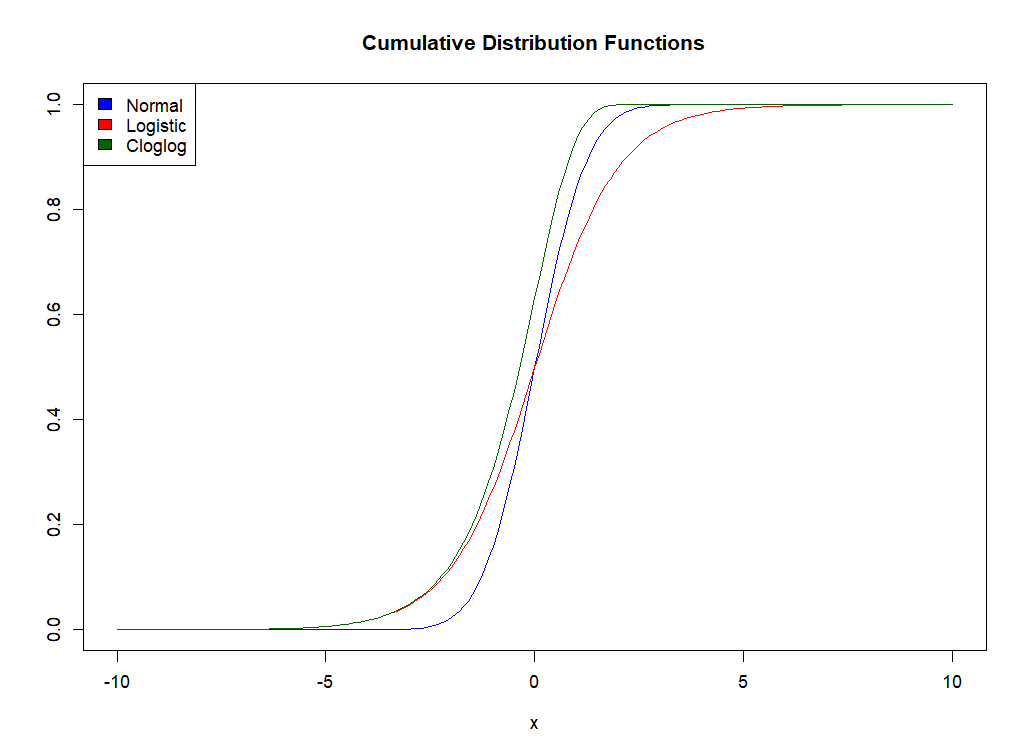
Logit and Probit Models

The logit and probit models deal explicitly with \(\color{darkblue}y\) being binary. They are closely related. The underlying probability models are:

\[\rm{Prob}(Y=1|\bf{x}) = \begin{cases} \Phi(\bf{x}'\bf{\beta}) & \text{for the probit model} \\ \Lambda(\bf{x}'\bf{\beta}) & \text{for the logit model}\end{cases}\] where \(\Phi(.)\) and \(\Lambda(.)\) are the normal and logistic distribution functions. 

In the text below, I use \[{\color{darkblue}{\bf x}}_i'{\color{darkred}\beta}\equiv\sum_j \color{darkblue}X_{i,j}\color{darkred}\beta_j\]

The standard way to estimate the coefficients is to form a log-likelihood function and maximize that. The likelihood function is \[\color{darkred}L=\prod_i F({\color{darkblue}{\bf x}}_i'{\color{darkred}\beta})^{\color{darkblue}y_i}\cdot [1-F(\color{darkblue}{\bf x}_i'\color{darkred}\beta)]^{1-\color{darkblue}y_i}\] So, the log-likelihood function is: \[\ln L = \sum_i \left\{\color{darkblue}y_i \ln F({\color{darkblue}{\bf x}}_i'{\color{darkred}\beta}) + (1-\color{darkred}y_i)\ln [1-F({\color{darkblue}{\bf x}}_i'{\color{darkred}\beta})]  \right\}\]

For the logit model, we have \[F(x) = \Lambda(x) = \frac{\exp(x)}{1+\exp(x)}\] Another way of writing this is \[F(x) = \frac{1}{1+\exp(-x)}\] The distribution function is \[f(x) = \Lambda(x)\left[1-\Lambda(x)\right]\] This is also often written as \[f(x)=\frac{\exp(-x)}{(1+\exp(-x))^2}=\frac{\exp(x)}{(1+\exp(x))^2}\] Plugging this in and after simplifying a bit, we end up with

Logit Log Likelihood
\[\max \ln \color{darkred}L = \sum_i \left\{\color{darkblue}y_i {\color{darkblue}{\bf x}}_i'{\color{darkred}\beta} - \ln\left[1+\exp({\color{darkblue}{\bf x}}_i'{\color{darkred}\beta})\right]\right\}\]

The first-order conditions of this form the following system of non-linear equations:

Logit First-Order Conditions
\[\sum_i \left[ \left(\color{darkblue}y_i-\frac{\exp({\color{darkblue}{\bf x}}_i'{\color{darkred}\beta})}{1+\exp({\color{darkblue}{\bf x}}_i'{\color{darkred}\beta})} \right) \color{darkblue}X_{i,j}\right] = 0 \>\>\>\forall j \]

The probit model can be stated directly as:

Probit Log Likelihood
\[\max \ln\color{darkred}L = \sum_i \left\{\color{darkblue}y_i \ln \Phi({\color{darkblue}{\bf{x}}}_i'{\color{darkred}{\bf{\beta}}}) + (1-\color{darkblue}y_i) \ln(1- \Phi({\color{darkblue}{\bf{x}}}_i'{\color{darkred}{\bf{\beta}}})) \right\}\]

where \(\Phi(.)\) is the error function. Not much simplification we can do here.

In these models, we repeat the expression \({\bf{x}}_i'{\bf{\beta}}\). Usually, I am inclined to prevent this, at the cost of an extra variable and equality constraint. In this case, it is most likely better just to keep the duplication: the summation length is small, and the cost of adding a constraint can be rather big. 

Another possible problem is that we may need to protect the \(\ln(x)\). Often we need to add \(x\gt 0\), or rather \(x\ge\mathit{tol}\) for a small constant \(\mathit{tol}\). In these formulations, we can safely ignore that as the argument of the \(\ln(x)\) function in reality never becomes zero or smaller.

I also reproduced the more exotic complementary log log model. This uses the distribution \[F(x) = 1-\exp[-\exp(x)]\] and \[f(x)=\exp(x)\exp[-\exp(x)]\] I could not find much information on the Gompertz model (except that the name is sometimes used for the CLogLog model). The Gompertz columns in table 17.1 from [1] remain a bit of a mystery to me.

Note that the Cloglog density is not symmetric while the probit (normal) and logit models are.

The final results table looks like:

----    497 PARAMETER results  replicate Greene table 17.1 

               OLS(QP1)    OLS(QP2)   OLS(NRML)     OLS(py)      LOGIT1
                  coeff       coeff       coeff       coeff       coeff

constant         -1.498      -1.498      -1.498      -1.498     -13.021
gpa               0.464       0.464       0.464       0.464       2.826
tuce              0.010       0.010       0.010       0.010       0.095
psi               0.379       0.379       0.379       0.379       2.379

          +      LOGIT2       LOGIT      PROBIT      PROBIT     CLOGLOG
                  coeff         APE       coeff         APE       coeff

constant        -13.021                  -7.452                 -10.031
gpa               2.826       0.363       1.626       0.361       2.294
tuce              0.095       0.012       0.052       0.011       0.041
psi               2.379       0.358       1.426       0.374       1.562
mean f(x'b)                   0.128                   0.222

          +     CLOGLOG
                    APE

gpa               0.413
tuce              0.007
psi               0.312
mean f(x'b)       0.180

It looks like we can reproduce the results in table 17.1 (apart from the Gompertz model). That is always reassuring. Being able to reproduce results is not always a given.

The logit model is better known as logistic regression, which has become quite popular in machine learning applications. 

Why log-likelihood?

One obvious question is: why do we use a log-likelihood function? One reason can be that the function is a bit easier to work with (e.g. differentiation is a bit simpler). There is also another reason.

The max likelihood objective is \[\max\>\color{darkred}L=\prod_i F({\color{darkblue}{\bf x}}_i'{\color{darkred}\beta})^{\color{darkblue}y_i}\cdot [1-F(\color{darkblue}{\bf x}_i'\color{darkred}\beta)]^{1-\color{darkblue}y_i}\] Note that \(\color{darkblue}y_i\in \{0,1\}\).

As an experiment, I use the following case:

• The probit model, with \(F(x)=\Phi(x)\) (i.e., the error function).
• Initial values for the coefficients: 0. This is the same as for the previous models.

This gives:

----    546 initial point

----    546 VARIABLE coeff.L  estimated coefficients

                      ( ALL       0.000 )


----    548 final point

----    548 VARIABLE coeff.L  estimated coefficients

                      ( ALL       0.000 )

 

So the solver did not move an inch! The initial point is returned as optimal solution. Let's investigate a bit.

This initial point coeff(p)=0 leads to an objective value that is essentially zero. Furthermore, the gradients are almost zero. Something we can verify by looking at the equation listing:

---- like  =E=  

like..  (1.85771975853216E-9)*coeff(constant) + (4.50125497492343E-9)*coeff(gpa)
     
      + (3.41820435569918E-8)*coeff(tuce) - (3.71543951706432E-10)*coeff(psi)
     
      + likelihood =E= 0 ;
     
      (LHS = -2.3283064365387E-10, INFES = 2.3283064365387E-10 ****)

  

The numbers in parentheses are gradients. If we compare this with the log-likelihood probit model (using the same starting point) we see:

 

---- probitObj  =E=  log likehood for Probit model

probitObj..  (7.97884560802865)*coeff(constant) + (19.3327429082534)*coeff(gpa)
     
      + (146.810759187727)*coeff(tuce) - (1.59576912160573)*coeff(psi) + lnL
      =E= 0 ; (LHS = 9.29107555578682, INFES = 9.29107555578682 ****)
     

This gives better-scaled gradients. That will cause the solver to actually move away from the initial point and search for better ones. 

Note that the INFES numbers in these sections are not something to worry about. This means that for the initial point coeff, the current values of likelihood and lnL are not correct. As this is the objective function, that is not an issue: the objective variable will be substituted out before solving starts.

Conclusion

I find that reproducing results of papers, book chapters, and the like, using a GAMS model is often a good exercise. It is my preferred way of reading such texts. There may be more easy-to-use canned routines for this in different statistical packages, but here we can verify the original mathematical formulation. 

We have discussed:

• Different formulations/tools for linear regression.
• Max log likelihood formulations for logit, probit, and complementary log log models.
• Implementation of partial effects (a.k.a. marginal effects).
• Issues with maximizing the likelihood function directly. 

 

References

1. William Greene, Econometric Analysis, 8th edition, 2017. Chapter 17, Binary Outcomes and Discrete Choices.
2. Spector, Lee C., and Michael Mazzeo. “Probit Analysis and Economic Education.” The Journal of Economic Education 11, no. 2 (1980): 37–44.

Appendix: GAMS model

$ontext    Discrete Choice Models    Reproduce table 17.1 in Greene, Econometric Analysis, 8th edition.    Data is from:       http://pages.stern.nyu.edu/~wgreene/Text/tables/TableF21-1.txt    Erwin Kalvelagen, Amsterdam Optimization $offtext option qcp=cplex, nlp=conopt; *----------------------------------------------------------- * raw data from Greene *----------------------------------------------------------- sets   i 'records' /case1*case32/   p0 'all variables' /constant,grade,gpa,tuce,psi/ ; table data(i,p0) 'raw data'             GPA      TUCE    PSI    GRADE  case1      2.66      20      0        0  case2      2.89      22      0        0  case3      3.28      24      0        0  case4      2.92      12      0        0  case5      4.00      21      0        1  case6      2.86      17      0        0  case7      2.76      17      0        0  case8      2.87      21      0        0  case9      3.03      25      0        0 case10      3.92      29      0        1 case11      2.63      20      0        0 case12      3.32      23      0        0 case13      3.57      23      0        0 case14      3.26      25      0        1 case15      3.53      26      0        0 case16      2.74      19      0        0 case17      2.75      25      0        0 case18      2.83      19      0        0 case19      3.12      23      1        0 case20      3.16      25      1        1 case21      2.06      22      1        0 case22      3.62      28      1        1 case23      2.89      14      1        0 case24      3.51      26      1        0 case25      3.54      24      1        1 case26      2.83      27      1        1 case27      3.39      17      1        1 case28      2.67      24      1        0 case29      3.65      21      1        1 case30      4.00      23      1        1 case31      3.10      21      1        0 case32      2.39      19      1        1 ; display data; *----------------------------------------------------------- * extract data * form y, x *----------------------------------------------------------- set p(p0) 'independent variables' /constant,gpa,tuce,psi/; parameters  y(i)    'dependent variable (grade)'  X(i,p)  'independent variables' ; y(i)   = data(i,'grade'); x(i,p) = data(i,p); x(i,'constant') = 1; display y,x; * check the assumption that y(i) is binary abort$sum(i$(y(i)<>0 and y(i)<>1),1) "GRADE should be binary"; * psi is binary is used in APE calculation abort$sum(i$(x(i,'psi')<>0 and x(i,'psi')<>1),1) "PSI should be binary"; *----------------------------------------------------------- * solve OLS as QP *----------------------------------------------------------- parameter results(*,*,*) 'replicate Greene table 17.1 '; option results:3:1:2; variable   sse        'sum of squared errors'   coeff(p)   'estimated coefficients'   e(i)       'error term' ; equation   obj        'objective'   fit(i)     'linear fit' ; obj..    sse =e= sum(i, sqr(e(i))); fit(i).. y(i) =e= sum(p, coeff(p)*x(i,p)) + e(i); model ols /obj,fit/; solve ols using qcp minimizing sse; results(p,'OLS(QP1)','coeff') = coeff.l(p); display results; *----------------------------------------------------------- * solve OLS as QP (alternative formulation) *----------------------------------------------------------- equation unconobj 'unconstrained objective'; unconobj.. sse =e= sum(i, sqr(y(i)-sum(p, coeff(p)*x(i,p)))); model ols2 /unconobj/; solve ols2 using qcp minimizing sse; results(p,'OLS(QP2)','coeff') = coeff.l(p); display results; *----------------------------------------------------------- * solve OLS as as system of linear equations * * solve the normal equations * * (X'X) b = X'y * *----------------------------------------------------------- alias(p,pp); parameter xx(p,pp) "inner product (X'X)"; xx(p,pp) = sum(i, x(i,p)*x(i,pp)); equation normal(p) 'normal equations'; normal(p).. sum(pp, xx(p,pp)*coeff(pp)) =e= sum(i, x(i,p)*y(i)); model ols3 /normal/; solve ols3 using cns; results(p,'OLS(NRML)','coeff') = coeff.l(p); display results; *----------------------------------------------------------- * solve OLS using python/numpy *----------------------------------------------------------- parameter theta(p) 'estimated coefficients'; $libinclude linalg ols i p x y theta results(p,'OLS(py)','coeff') = theta(p); display results; *----------------------------------------------------------- * Logit model 1 : optimization *----------------------------------------------------------- variable lnL 'log likelihood'; equation LogitObj 'log likelihood for Logit model'; LogitObj.. lnL =e= sum(i, y(i)*sum(p, coeff(p)*x(i,p))                        - log[1 + exp(sum(p, coeff(p)*x(i,p)))]                     ); model logit1 /LogitObj/; * reset levels (no cheating) coeff.l(pp)=0; solve logit1 using nlp maximizing lnL; results(p,'LOGIT1','coeff') = coeff.l(p); display results; *----------------------------------------------------------- * Logit model 2 : system of equations *----------------------------------------------------------- alias(p,pp); equation LogitFirstOrder 'Logit first order conditions'; LogitFirstOrder(p)..    sum(i, {y(i)-exp(sum(pp, coeff(pp)*x(i,pp)))/                [1+exp(sum(pp, coeff(pp)*x(i,pp)))]}*x(i,p)) =e= 0; model logit2 /LogitFirstOrder/; * reset levels coeff.l(pp)=0; solve logit2 using cns; results(p,'LOGIT2','coeff') = coeff.l(p); display results; *----------------------------------------------------------- * Logit APE *----------------------------------------------------------- set pnoc(p) 'p except const'; pnoc(p) = not sameas(p,'constant'); parameter xb(i) 'Xb (intermediate expression)'; Xb(i) = sum(p, coeff.l(p)*x(i,p)); results(pnoc,'LOGIT','APE') =   sum(i, exp(Xb(i))/sqr(1+exp(Xb(i)))*coeff.l(pnoc))/card(i); parameter xb2(i,*) 'Xb2 (Xb with PSI=0 and PSI=1)'; xb2(i,'PSI=0') = sum(p$(not sameas(p,'PSI')), coeff.l(p)*x(i,p)); xb2(i,'PSI=1') = xb2(i,'PSI=0')+coeff.l('PSI'); parameter plogis(i,*) 'logistic distribution'; plogis(i,'PSI=1') = 1/(1+exp(-xb2(i,'PSI=1'))); plogis(i,'PSI=0') = 1/(1+exp(-xb2(i,'PSI=0'))); results('PSI','LOGIT','APE') =   sum(i,plogis(i,'PSI=1')-plogis(i,'PSI=0'))/card(i); results("mean f(x'b)",'LOGIT','APE') =   sum(i, exp(Xb(i))/sqr(1+exp(Xb(i))))/card(i); display plogis,Xb2 display results; *----------------------------------------------------------- * Probit model *----------------------------------------------------------- equation probitObj 'log likehood for Probit model'; probitObj..    lnL =e= sum(i, y(i)*log(errorf(sum(p, coeff(p)*x(i,p)))) +                   (1-y(i))*log(1-errorf(sum(p, coeff(p)*x(i,p))))); model probit /probitObj/; * reset levels coeff.l(pp)=0; solve probit maximizing lnL using nlp; results(p,'PROBIT','coeff') = coeff.l(p); results(pnoc,'PROBIT','APE') =   sum(i, 1/sqrt(2*pi) * exp(-0.5*sqr(sum(p, coeff.l(p)*x(i,p)))) * coeff.l(pnoc))/card(i); * same as for logit APE xb2(i,'PSI=0') = sum(p$(not sameas(p,'PSI')), coeff.l(p)*x(i,p)); xb2(i,'PSI=1') = xb2(i,'PSI=0')+coeff.l('PSI'); results('PSI','PROBIT','APE') = sum(i, errorf(xb2(i,'PSI=1'))-errorf(xb2(i,'PSI=0')))/card(i); results("mean f(x'b)",'PROBIT','APE') =   sum(i, 1/sqrt(2*pi) * exp(-0.5*sqr(sum(p, coeff.l(p)*x(i,p)))))/card(i); display results; *----------------------------------------------------------- * Complementary log log model *----------------------------------------------------------- equation compLogLogObj 'log likehood for comp log log model'; compLogLogObj..    lnL =e= sum(i, y(i)*log(1-exp(-exp(sum(p, coeff(p)*x(i,p))))) +                   (1-y(i))*log(exp(-exp(sum(p, coeff(p)*x(i,p)))))); model comploglog /compLogLogObj/; * reset levels coeff.l(pp)=0; solve comploglog maximizing lnL using nlp; results(p,'CLOGLOG','coeff') = coeff.l(p); Xb(i) = sum(p, coeff.l(p)*x(i,p)); results(pnoc,'CLOGLOG','APE') =   sum(i, exp(Xb(i))*exp(-exp(Xb(i))) * coeff.l(pnoc))/card(i); * same as for logit APE xb2(i,'PSI=0') = sum(p$(not sameas(p,'PSI')), coeff.l(p)*x(i,p)); xb2(i,'PSI=1') = xb2(i,'PSI=0')+coeff.l('PSI'); results('PSI','CLOGLOG','APE') = sum(i, exp(-exp(xb2(i,'PSI=0')))-exp(-exp(xb2(i,'PSI=1'))))/card(i); results("mean f(x'b)",'CLOGLOG','APE') =   sum(i, exp(Xb(i))*exp(-exp(Xb(i))))/card(i); display results; *----------------------------------------------------------- * Gompertz model *----------------------------------------------------------- $onText Don't know how to do this. Often the cloglog model is stated to have an underlying Gompertz model. The cloglog model uses    f(x) = exp(x)*exp(-exp(x)) This is the same as    f(x) = exp(x-exp(x)) This is the Gompertz pdf (see https://en.wikipedia.org/wiki/Gompertz_distribution). $offText *----------------------------------------------------------- * Why log likelihood? *----------------------------------------------------------- $onText   Instead of maximizing the log likelihood function we try   here to maximize the likelihood function of the probit model   directly.   The gradients are so small, that solvers stop at the initial   point and don't move an inch. $offText variable likelihood; equation like; like.. likelihood =e=      prod(i,power(errorf(sum(p,coeff(p)*x(i,p))),y(i))             * power(1-errorf(sum(p,coeff(p)*x(i,p))),1-y(i))); model probit2 /like/; coeff.l(p) = 0.0; display "initial point",coeff.l; solve probit2 maximizing likelihood using nlp; display "final point",coeff.l;