I am teaching some GAMS classes this summer. The first class is about the transportation model. This is model number 1 from the GAMS model library [1]. It is a tiny model, slightly modified from the original model in [2]. I believe the GAMS version has been made dual degenerate.
The model is really very small (2 supply nodes, 3 demand nodes). To show that GAMS and the Cplex LP solver are designed and built for large models, I often do the following exercise. Create a set \(k\) with 10, or 100, or 1000 elements. Then replace all \(\color{darkred}x_{i,j}\) by \(\color{darkred}x_{i,j,k}\). And similar for the demand supply constraint blocks. The objective becomes \[\color{darkred}z=\sum_{i,j,k}\color{darkblue}c_{i,j}\cdot\color{darkred}x_{i,j,k}\] We have now duplicated the original small LP to a large block-diagonal structure:
(to be precise: it is block-diagonal after reordering).
| Transportation Model | Augmented Model |
|---|---|
| \[\begin{align}\min&\sum_{i,j}\color{darkblue}c_{i,j}\cdot\color{darkred}x_{i,j}\\ & \sum_j \color{darkred}x_{i,j} \le \color{darkblue}a_i && \forall i \\& \sum_i \color{darkred}x_{i,j} \ge \color{darkblue}b_j && \forall j \\ & \color{darkred}x_{i,j} \ge 0 \end{align}\] | \[\begin{align}\min&\sum_{i,j,k}\color{darkblue}c_{i,j}\cdot\color{darkred}x_{i,j,k}\\ & \sum_j \color{darkred}x_{i,j,k} \le \color{darkblue}a_i && \forall i,k \\& \sum_i \color{darkred}x_{i,j,k} \ge \color{darkblue}b_j && \forall j,k \\ & \color{darkred}x_{i,j,k} \ge 0 \end{align} \] |
----     75 PARAMETER report

                     1          10         100        1000       10000      100000

variables        7.000      61.000     601.000    6001.000   60001.000  600001.000
equations        6.000      51.000     501.000    5001.000   50001.000  500001.000
nonzeros        19.000     181.000    1801.000   18001.000  180001.000 1800001.000
obj            153.675    1536.750   15367.500  153675.000 1536750.000 1.536750E+7
iterations       4.000       4.000       4.000       4.000       3.000       3.000
time             0.032                   0.016       0.032       0.093       1.094
The table shows how the model grows when we increase the size of the set \(k\). The presolve seems to keep most of the model:
Tried aggregator 1 time.
LP Presolve eliminated 0 rows and 1 columns.
Reduced LP has 500000 rows, 600000 columns, and 1200000 nonzeros.
Presolve time = 0.38 sec. (505.30 ticks)
Symmetry aggregator did 1099989 additional substitutions.

Iteration log . . .
Iteration:     1   Dual objective     =       7312499.999993

Dual crossover.
  Dual:  Fixed no variables.
  Primal:  Fixed no variables.

--- LP status (1): optimal.
--- Cplex Time: 0.69sec (det. 1174.36 ticks)
although I don't know exactly what a symmetry aggregator does. Note: all runs were with default settings using 1 thread.
I don't have a good explanation for the iteration counts. I expected them to grow somewhat. Staying flat would be excellent. But decreasing is a bit of a surprise. Certainly, some other solvers I tried did not achieve this.
One complication is that Cplex decides on what LP solver to use. It looks like for \(k=1\) Cplex uses dual simplex, and for the others, it uses the barrier algorithm (a.k.a. interior-point algorithm). A little bit of guesswork is involved here, as the log is not very clear on this. The line Dual crossover may indicate a barrier method was used. Note that the Simplex Method typically needs many, cheap iterations, and the barrier uses few but more expensive iterations. I suspect or guess that for the very large problems Cplex may stop a bit earlier because the objective becomes so large: some relative stopping criterion may be easier to hit. Simplex methods use an absolute optimality tolerance (independent of the data), while barrier methods use a relative convergence tolerance (depends on the data).
For comparison, a different high-end solver showed:
----     79 PARAMETER report

                     1          10         100        1000       10000

variables        7.000      61.000     601.000    6001.000   60001.000
equations        6.000      51.000     501.000    5001.000   50001.000
nonzeros        19.000     181.000    1801.000   18001.000  180001.000
obj            153.675    1536.750   15367.500  153675.000 1536750.000
iterations       4.000      40.000     107.000    1007.000   10007.000
time             0.012       0.009       0.012       0.030       0.273

         +      100000

variables   600001.000
equations   500001.000
nonzeros   1800001.000
obj        1.536750E+7
iterations  100007.000
time             2.930
I assume this was using Dual Simplex for all LPs (using 1 thread). Note: Don't compare the timings between the solvers: this was run on a different machine.
I know this is a somewhat silly experiment. But I like it: adding an index this way is something that happens on more occasions. And we demonstrate we can do large models quickly (well, transportation LPs are about the easiest LPs in existence). And as it turns out: the performance figures we see can be a bit of a mystery.
Conclusion
Model number 1 of the GAMS model library is more interesting than you might guess.
References
- trnsport.gms: A Transportation Problem, https://www.gams.com/latest/gamslib_ml/libhtml/gamslib_trnsport.html
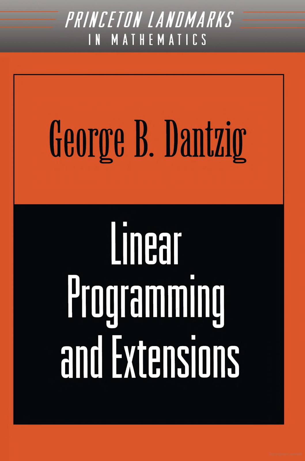
- George B. Dantzig, Linear Programming and Extensions, Princeton University Press, 1963.
Appendix: GAMS model
|
$ontext |


No comments:
Post a Comment