This is a follow-up on the post on the max sum submatrix problem [1]. There we looked at the problem of finding a contiguous submatrix that maximizes the sum of the values in this submatrix.
A little bit more complicated is the following continuous version of this problem.
Assume we have \(n\) points with an \(x\)- and \(y\)-coordinate and a value. Find the rectangle such that the sum of the values of all points inside is maximized.
Data set
I generated a random data set with \(n=100\) points:
----     10 PARAMETER p  points

               x           y       value

i1        17.175       5.141       8.655
i2        84.327       0.601      -3.025
i3        55.038      40.123      -9.834
i4        30.114      51.988       8.977
i5        29.221      62.888       1.438
i6        22.405      22.575      -3.327
i7        34.983      39.612       9.675
i8        85.627      27.601       5.329
i9         6.711      15.237      -7.798
i10       50.021      93.632       9.896
i11       99.812      42.266       1.606
i12       57.873      13.466      -6.672
i13       99.113      38.606       2.867
i14       76.225      37.463      -3.114
i15       13.069      26.848       8.247
i16       63.972      94.837       8.001
i17       15.952      18.894      -9.675
i18       25.008      29.751      -2.627
i19       66.893       7.455       3.288
i20       43.536      40.135       1.868
i21       35.970      10.169      -9.309
i22       35.144      38.389       6.836
i23       13.149      32.409       8.642
i24       15.010      19.213       0.159
i25       58.911      11.237      -4.008
i26       83.089      59.656      -0.068
i27       23.082      51.145      -9.101
i28       66.573       4.507       5.474
i29       77.586      78.310       0.659
i30       30.366      94.575       4.935
i31       11.049      59.646       4.401
i32       50.238      60.734       2.632
i33       16.017      36.251      -7.702
i34       87.246      59.407       9.423
i35       26.511      67.985       4.135
i36       28.581      50.659       9.725
i37       59.396      15.925       7.096
i38       72.272      65.689       2.429
i39       62.825      52.388       4.026
i40       46.380      12.440       4.018
i41       41.331      98.672       5.814
i42       11.770      22.812       2.204
i43       31.421      67.565      -8.914
i44        4.655      77.678      -0.296
i45       33.855      93.245      -8.949
i46       18.210      20.124       3.972
i47       64.573      29.714      -6.104
i48       56.075      19.723      -5.479
i49       76.996      24.635       6.273
i50       29.781      64.648       9.835
i51       66.111      73.497       5.013
i52       75.582       8.544       4.367
i53       62.745      15.035      -9.988
i54       28.386      43.419      -4.723
i55        8.642      18.694       6.476
i56       10.251      69.269       6.391
i57       64.125      76.297       7.208
i58       54.531      15.481      -5.746
i59        3.152      38.938      -0.864
i60       79.236      69.543      -9.233
i61        7.277      84.581      -3.540
i62       17.566      61.272      -1.202
i63       52.563      97.597      -3.693
i64       75.021       2.689      -7.305
i65       17.812      18.745       6.219
i66        3.414       8.712      -1.664
i67       58.513      54.040      -7.164
i68       62.123      12.686      -0.689
i69       38.936      73.400      -4.340
i70       35.871      11.323       7.914
i71       24.303      48.835      -8.712
i72       24.642      79.560      -1.708
i73       13.050      49.205      -3.168
i74       93.345      53.356      -0.634
i75       37.994       1.062       2.853
i76       78.340      54.387       2.872
i77       30.003      45.113      -3.248
i78       12.548      97.533      -7.984
i79       74.887      18.385       8.117
i80        6.923      16.353      -5.653
i81       20.202       2.463       8.377
i82        0.507      17.782      -0.965
i83       26.961       6.132      -8.201
i84       49.985       1.664      -2.516
i85       15.129      83.565      -1.700
i86       17.417      60.166      -1.916
i87       33.064       2.702      -7.767
i88       31.691      19.609       5.023
i89       32.209      95.071       6.068
i90       96.398      33.554      -9.527
i91       99.360      59.426      -0.382
i92       36.990      25.919      -4.428
i93       37.289      64.063       8.032
i94       77.198      15.525      -9.648
i95       39.668      46.002       3.621
i96       91.310      39.334       9.018
i97       11.958      80.546       8.004
i98       73.548      54.099       7.976
i99        5.542      39.072       7.489
i100      57.630      55.782      -2.180

High-level model
Let's denote our points by: \(\color{darkblue}p_{i,a}\), where \(a=\{x,y,{\mathit{value}}\}\). Our decision variables are the corner points of the rectangle: \(\color{darkred}r_{c,q}\) where \(c=\{x,y\}\) and \(q=\{min,max\}\). These variables are continuous between \(\color{darkblue}L=0\) and \(\color{darkblue}U=100\).
| High-level model |
|---|
| \[\begin{align}\max & \sum_{i|\color{darkred}r(c,min) \le \color{darkblue}p(i,c)\le \color{darkred}r(c,max)} \color{darkblue}p_{i,{\mathit{value}}}\\ & \color{darkred}r_{c,min} \le \color{darkred}r_{c,max} \\ &\color{darkred}r_{c,q}\in [L,U]\end{align}\] |
This looks easy. Well, not so fast...
Development
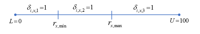
The first thing to do is to introduce binary variables that indicate if a point \(i\) is in between \(\color{darkred}r_{c,min}\) and \(\color{darkred}r_{c,max}\) for both \(c \in \{x,y\}\). It is actually simpler to consider three cases:
The \(x\)-coordinate of a given point \(\color{darkblue}p_{i,x}\) is in one of the three segments denoted by \(\color{darkred}\delta_{i,x,k}\). Of course, similar for the \(y\)-coordinate. Note that this is a little bit different than usual. Normally we have a point which is a decision variable and the limits for the segments that are constants. Here we have a fixed data point, but the segment boundaries \(\color{darkred}r_{x,min}, \color{darkred}r_{x,max}\) are variable.
So, looking at the picture, we need to implement: \[\begin{align} &\color{darkred}\delta_{i,x,1}=1 \Rightarrow \color{darkblue}L \le \color{darkblue} p_{i,x} \le \color{darkred}r_{x,min} \\ & \color{darkred}\delta_{i,x,2}=1 \Rightarrow \color{darkred}r_{x,min} \le \color{darkblue}p_{i,x} \le \color{darkred}r_{x,max} \\ &\color{darkred}\delta_{i,x,3}=1\Rightarrow \color{darkred}r_{x,max} \le \color{darkblue} p_{i,x} \le \color{darkblue}U \\ & \sum_k \color{darkred}\delta_{i,x,k}= 1\end{align}\] We can formulate the implications as the following inequalities: \[\begin{align} &\color{darkred}r_{x,min} \ge \color{darkblue}p_{i,x} \cdot \color{darkred}\delta_{i,x,1} + \color{darkblue}L \cdot (1-\color{darkred}\delta_{i,x,1}) \\ & \color{darkred}r_{x,min} \le \color{darkblue} p_{i,x} \cdot \color{darkred}\delta_{i,x,2} + \color{darkblue}U \cdot (1-\color{darkred}\delta_{i,x,2}) \\& \color{darkred}r_{x,max} \ge \color{darkblue}p_{i,x} \cdot \color{darkred}\delta_{i,x,2} + \color{darkblue}L \cdot (1-\color{darkred}\delta_{i,x,2}) \\ & \color{darkred}r_{x,max} \le \color{darkblue} p_{i,x} \cdot \color{darkred}\delta_{i,x,3} + \color{darkblue}U \cdot (1-\color{darkred}\delta_{i,x,3})\end{align}\]
Of course, we need to repeat this for the \(y\) direction. Once we have all variables \(\color{darkred}\delta_{i,x,k}\) and \(\color{darkred}\delta_{i,y,k}\), we still need to combine them. A point \(i\) is inside the rectangle \(\color{darkred}r\) if and only if \(\color{darkred}\delta_{i,x,2}\cdot \color{darkred}\delta_{i,y,2} = 1\).
With this, our model can look like:
| MIQP Model A |
|---|
| \[\begin{align}\max & \sum_i \color{darkblue}p_{i,{\mathit{value}}} \cdot \color{darkred}\delta_{i,x,2} \cdot \color{darkred}\delta_{i,y,2}\\ &
\color{darkred}r_{c,min} \ge \color{darkblue} p_{i,c} \cdot \color{darkred}\delta_{i,c,1} + \color{darkblue}L \cdot (1-\color{darkred}\delta_{i,c,1}) && \forall i,c\\ & \color{darkred}r_{c,{\mathit{min}}} \le \color{darkblue} p_{i,c} \cdot \color{darkred}\delta_{i,c,2} + \color{darkblue}U \cdot (1-\color{darkred}\delta_{i,c,2}) && \forall i,c\\& \color{darkred}r_{c,{\mathit{max}}} \ge \color{darkblue} p_{i,c} \cdot \color{darkred}\delta_{i,c,2} + \color{darkblue}L \cdot (1-\color{darkred}\delta_{i,c,2}) && \forall i,c \\ & \color{darkred}r_{c,{\mathit{max}}} \le \color{darkblue} p_{i,c} \cdot \color{darkred}\delta_{i,c,3} + \color{darkblue}U \cdot (1-\color{darkred}\delta_{i,c,3}) &&\forall i,c \\ & \sum_k \color{darkred}\delta_{i,c,k}=1 && \forall i,c \\ & \color{darkred}r_{c,min} \le \color{darkred}r_{c,max} && \forall c \\ & \color{darkred}\delta_{i,c,k} \in \{0,1\} \\ &\color{darkred}r_{c,q} \in [\color{darkblue}L,\color{darkblue}U] \end{align}\] |
This model can easily be linearized using the techniques demonstrated in [1]. Here we will assume the solver is linearizing this automatically. This model solves very quickly, and the results are:
----     62 VARIABLE z.L                   =      102.234  objective

----     62 VARIABLE r.L  rectangle

          min         max

x       7.277      93.345
y      15.525      97.533
The solver (Cplex in this case), linearized the problem for us and solved it as a linear MIP. It found and proved the global optimal solution in 0 nodes (i.e. all work was done during preprocessing) and 1,249 iterations. The solution time was 2 seconds.
Alternative approach
In the comments, Imre Polik suggested populating a (very) sparse matrix using the values and then apply a method from [1]. The sparse matrix has one element per row and column, and the points are sorted by their \(x\)- and \(y\)-coordinate. The following small example shows how this is done:
----     17 PARAMETER pt  points

              x           y       value

i1       17.175      99.812      -2.806
i2       84.327      57.873      -2.971
i3       55.038      99.113      -7.370
i4       30.114      76.225      -6.998
i5       29.221      13.069       1.782
i6       22.405      63.972       6.618
i7       34.983      15.952      -5.384
i8       85.627      25.008       3.315
i9        6.711      66.893       5.517
i10      50.021      43.536      -3.927


----     52 PARAMETER spMap  sparse matrix mapper

                      x           y       value

i1 .i2 .i10      17.175      99.812      -2.806
i2 .i9 .i5       84.327      57.873      -2.971
i3 .i8 .i9       55.038      99.113      -7.370
i4 .i5 .i8       30.114      76.225      -6.998
i5 .i4 .i1       29.221      13.069       1.782
i6 .i3 .i6       22.405      63.972       6.618
i7 .i6 .i2       34.983      15.952      -5.384
i8 .i10.i3       85.627      25.008       3.315
i9 .i1 .i7        6.711      66.893       5.517
i10.i7 .i4       50.021      43.536      -3.927


----     56 PARAMETER spA  sparse matrix representation

             i1          i2          i3          i4          i5          i6          i7          i8          i9         i10

i1                                                                                5.517
i2                                                                                                                   -2.806
i3                                                                    6.618
i4        1.782
i5                                                                                           -6.998
i6                   -5.384
i7                                           -3.927
i8                                                                                                       -7.370
i9                                                       -2.971
i10                               3.315
The first parameter holds our points. The second parameter shows the mapping between the original record number (column one) and the location in the matrix \((i,j)\): the second and third index. The final parameter shows the matrix in a more standard representation. (Note: this is not so easy to do in GAMS. You could use
gdxrank. I used a little bit of Python code to do the sorting.) With this we can use the model from [1]:
| MIQP model B |
|---|
| \[\begin{align} \max& \sum_{i,j} \color{darkblue}a_{i,j} \cdot \color{darkred}x_i \cdot \color{darkred}y_j\\ & \color{darkred}p_i \ge \color{darkred}x_{i} - \color{darkred}x_{i-1} \\ & \color{darkred}q_j \ge \color{darkred}y_{j} - \color{darkred}y_{i-1} \\ & \sum_i \color{darkred}p_i \le 1 \\ & \sum_j \color{darkred}q_j \le 1\\ &\color{darkred}x_i, \color{darkred}y_j,\color{darkred}p_i, \color{darkred}q_j \in \{0,1\} \end{align}\] |
We assume \(\color{darkred}x_0 = \color{darkred}y_0= 0\). Of course, we can apply a standard linearization or let the solver linearize. Note that we only have \(n\) quadratic terms (only for the nonzero elements). When we find the optimal solution for this model, we can retrieve the \(x\)- and \(y\)-coordinate of the first and last selected row and column to form our rectangle.
With our 100 point data set, we find the optimal solution in 0 nodes and 759 iterations. This took less than a second.
Genetic algorithm
Here we try to solve the problem using R's GA package. The fitness function is basically the same as our objective in the high-level model. The code (and output) can look like:
> library(GA)
>
> # data is stored in data frame
> str(df)
'data.frame':	100 obs. of  4 variables:
 $ point: chr  "i1" "i2" "i3" "i4" ...
 $ x    : num  17.2 84.3 55 30.1 29.2 ...
 $ y    : num  5.141 0.601 40.123 51.988 62.888 ...
 $ value: num  8.66 -3.02 -9.83 8.98 1.44 ...
>
> # fitness function
> f <- function(x) {
+   xmin <- min(x[1],x[2])
+   xmax <- max(x[1],x[2])
+   ymin <- min(x[3],x[4])
+   ymax <- max(x[3],x[4])
+   ok <- (df$x <= xmax) & (df$x >= xmin) & (df$y <= ymax) & (df$y >= ymin)
+   sum(ok * df$value)
+ }
>
> # call the ga solver
> system.time(result <- ga(type = "real-valued",
+                       fitness = f,
+                       lower = rep(0,4), upper = rep(100,4),
+                       popSize = 100, maxiter = 500, monitor = T,
+                       seed = 12345))
GA | iter = 1 | Mean =  8.058819 | Best = 48.175182
GA | iter = 2 | Mean =  6.413503 | Best = 48.175182
GA | iter = 3 | Mean =  8.234065 | Best = 48.175182
GA | iter = 4 | Mean =  5.209888 | Best = 48.175182
GA | iter = 5 | Mean =  7.171262 | Best = 48.175182
GA | iter = 6 | Mean =  9.767468 | Best = 48.175182
GA | iter = 7 | Mean = 11.41823 | Best = 48.17518
GA | iter = 8 | Mean =  9.89723 | Best = 48.20186
GA | iter = 9 | Mean = 14.19131 | Best = 53.02362
GA | iter = 10 | Mean = 20.83307 | Best = 53.61161
. . .
GA | iter = 490 | Mean =  87.13611 | Best = 102.23405
GA | iter = 491 | Mean =  83.61628 | Best = 102.23405
GA | iter = 492 | Mean =  87.16728 | Best = 102.23405
GA | iter = 493 | Mean =  86.52578 | Best = 102.23405
GA | iter = 494 | Mean =  83.02602 | Best = 102.23405
GA | iter = 495 | Mean =  86.58533 | Best = 102.23405
GA | iter = 496 | Mean =  89.53308 | Best = 102.23405
GA | iter = 497 | Mean =  89.4938 | Best = 102.2341
GA | iter = 498 | Mean =  88.29249 | Best = 102.23405
GA | iter = 499 | Mean =  88.39676 | Best = 102.23405
GA | iter = 500 | Mean =  85.33931 | Best = 102.23405
   user  system elapsed
   6.78    0.27    7.32
Note that I did not specify the constraints \(\color{darkred}{\mathit{xmin}} \le \color{darkred}{\mathit{xmax}}\) and \(\color{darkred}{\mathit{ymin}} \le \color{darkred}{\mathit{ymax}}\). Instead, when the fitness function receives the vector \(x\) it just sorts the values. This is somewhat of a trick. But it helps in allowing us to use an unconstrained optimization problem. Additionally, we have good bounds on the four decision variables. These properties are usually a big win for heuristic solvers like this.
Because we know the optimal solution, we can indeed verify that this heuristic also finds the optimal solution.
A nice feature is to plot the results:
It finds 5 solutions with the best objective:
> result@solution
           x1       x2       x3       x4
[1,] 8.058577 91.76226 15.88715 95.49885
[2,] 8.072476 91.76382 15.87492 95.50330
[3,] 8.086532 91.76143 15.91187 95.52999
[4,] 8.071193 91.76518 15.88455 95.50384
[5,] 7.978493 92.05050 15.92354 95.49153
These are essentially the same.
Larger data set
When using a larger random data set with \(n=1,000\) points, we end up with a large MIQP Model A. It has 10k rows and 6k columns. After Cplex reformulates this into a linear model, we have 11.5k rows and 7k columns. This solves to optimality in 2,000 seconds with a proven optimal objective of 209.426.
----     63 VARIABLE z.L                   =      209.426  objective

----     63 VARIABLE r.L  rectangle

          min         max

x       7.045      97.298
y       2.812      58.167
MIQP Model B is smaller. Before linearization, we have 2k rows and 4k columns. This translates to 3,495 rows, 4,982 columns after (automatic) linearization and presolving. The model solves in about 100 seconds and finds and proves the global optimum of 209.426.
----     88 VARIABLE z.L                   =      209.426  objective

----     98 PARAMETER results  model B results

              x           y

min       7.098       2.812
max      97.215      57.956
When I feed this into the GA solver, with a limit of 5,000 iterations, we see:
-- Genetic Algorithm -------------------

GA settings:
Type                  =  real-valued
Population size       =  10
Number of generations =  5000
Elitism               =  1
Crossover probability =  0.8
Mutation probability  =  0.1
Search domain =
       x1  x2  x3  x4
lower   0   0   0   0
upper 100 100 100 100

GA results:
Iterations             = 5000
Fitness function value = 205.203
Solutions =
           x1       x2      x3       x4
[1,] 80.91125 7.089162 58.0342 11.90685
[2,] 80.91125 7.089162 58.0342 11.90685
[3,] 80.91125 7.089162 58.0342 11.90685
[4,] 80.91125 7.089162 58.0342 11.90685
Note that in this case, \(x_1,x_2,x_3,x_4\) corresponds to \(xmax,xmin,ymax,ymin\).
We see that the \(x\) part of the rectangle is close, but \(ymin=11.9\) is a bit off compared to the optimal MIQP solution. Indeed the objective 205.203 is a little bit worse than 209.426 which we found earlier. On the other hand, GA just needed about 10 seconds to find this solution (depending on the population size).
Conclusions
- Formulating this problem as a non-convex MIQP model requires some thought (and some work).
- But it can provide proven optimal solutions (or good solutions if optimality is too costly).
- The sparse matrix formulation (model B) works better than the rectangle formulation (model A).
- Using a Genetic Algorithm based heuristic makes the modeling quite easy. There is one trick involved so we have an unconstrained problem. After that, the GA solver finds the optimal solution fairly quickly. Of course, it does not prove optimality. We only know this because we also have a mathematical programming model that was solved before.
- The GA model and the MIQP model have very little in common. It is almost always a bad idea to reuse a MIP model and feed it directly to a meta-heuristic.
- When developing heuristics for a large and difficult problem, I also like to implement a mathematical programming model. This allows us to compare solutions. First, this is a good debugging aid. But also this can give us some feedback on the quality of the solutions found with the heuristic, even if only for smaller data sets.
References
|
$ontext
Given:
n points with (x,y) coordinates and a value
(value
can be positive or negative).
Find a
rectangle such that the sum of the values of the
points
inside is maximized.
This
formulation works directly on the points. Each point
is in
one of three regions for each coordinate:
L -------- min -------- max --------- U
region: k1 k2 k3
$offtext
*----------------------------------------------------------------
* data
*----------------------------------------------------------------
set
i 'number of points' /i1*i100/
a 'attributes' /x,y,value/
c(a) 'coordinates' /x,y/
k 'segment' /k1 'before'
k2 'in
between'
k3 'after'/
q 'limit' /min,max/
;
*
* select (x,y) coordinates from [L,U]x[L,U]
*
scalars
L /0/
U /100/
;
parameter p(*,*) 'points';
p(i,'x') = uniform(L,U);
p(i,'y') = uniform(L,U);
p(i,'value') =
uniform(-10,10);
display p;
*----------------------------------------------------------------
* model
*----------------------------------------------------------------
variable
z 'objective'
r(c,q) 'rectangle'
;
r.lo(c,q) = L;
r.up(c,q) = U;
binary variable delta(c,i,k) 'region of point i';
equations
obj 'objective'
e1(c,i) 'region k1'
e2(c,i) 'region k2'
e3(c,i) 'region k2'
e4(c,i) 'region k3'
one(c,i) 'point is in one region'
minmax(c) 'min <= max'
;
obj.. z=e= sum(i, p(i,'value')*delta('x',i,'k2')*delta('y',i,'k2'));
e1(c,i).. r(c,'min') =g= p(i,c)*delta(c,i,'k1')+L*(1-delta(c,i,'k1'));
e2(c,i).. r(c,'min') =l= p(i,c)*delta(c,i,'k2')+U*(1-delta(c,i,'k2'));
e3(c,i).. r(c,'max') =g= p(i,c)*delta(c,i,'k2')+L*(1-delta(c,i,'k2'));
e4(c,i).. r(c,'max') =l= p(i,c)*delta(c,i,'k3')+U*(1-delta(c,i,'k3'));
one(c,i).. sum(k,delta(c,i,k)) =e= 1;
minmax(c).. r(c,'min') =l= r(c,'max');
model mod /all/;
option
optcr=0,threads=8,miqcp=cplex;
solve mod
maximizing z using miqcp;
display z.l,r.l;
|
Appendix B: GAMS formulation B
|
$ontext
Given:
n points with (x,y) coordinates and a value
(value
can be positive or negative).
Find a
rectangle such that the sum of the values of the
points
inside is maximized.
This
formulation sorts the points by x and y coordinates
to form
a (very) sparse matrix (one element per row and column).
$offtext
*------------------------------------------------------
* data
*------------------------------------------------------
set
i 'number of points' /i1*i100/
a 'attributes' /x,y,value/
c(a) 'coordinates' /x,y/
;
*
* select (x,y) coordinates from [L,U]x[L,U]
*
scalars
L /0/
U /100/
;
parameter pt(i,a) 'points';
pt(i,'x') = uniform(L,U);
pt(i,'y') = uniform(L,U);
pt(i,'value') =
uniform(-10,10);
display pt;
*------------------------------------------------------
* create a sparse matrix representation
*------------------------------------------------------
alias(i,j,k);
parameter
spMap(i,j,k,a) 'sparse
matrix mapper';
EmbeddedCode Python:
# copy pt to Python
p = gams.get("pt")
# index i
indx = [t[0][0] for t in p if t[0][1]=="x"]
n = len(indx)
# get x,y,value
x = [t[1] for t in p if t[0][1]=="x"]
y = [t[1] for t in p if t[0][1]=="y"]
v = [t[1] for t in p if t[0][1]=="value"]
# get rank of x,y
xrank = [sorted(x).index(i) for i in x]
yrank = [sorted(y).index(i) for i in y]
# create a parameter q that has x and y sorted
q = []
for k in range(n):
i0 = indx[k]
i = indx[xrank[k]]
j = indx[yrank[k]]
q.append((i0,i,j,"x",x[k]))
q.append((i0,i,j,"y",y[k]))
q.append((i0,i,j,"value",v[k]))
gams.set("spmap",q)
endEmbeddedCode spmap
option spmap:3:3:1;
display$(card(spmap)<=500) spmap;
parameter spA(i,j) 'sparse matrix
representation';
spA(i,j) = sum(k,spmap(k,i,j,'value'));
display$(card(spA)<=100) spA;
*------------------------------------------------------
* model
*------------------------------------------------------
binary variable
x(i) 'selected rows'
y(j) 'selected columns'
p(i) 'start of submatrix'
q(j) 'start of submatrix'
;
variable z 'objective';
equation
obj 'objective'
pbound 'x(i-1)=0,x(i)=1 => p(i)=1'
qbound 'y(i-1)=0,y(i)=1 => q(i)=1'
plim 'sum(p) <= 1'
qlim 'sum(q) <= 1'
;
* objective is linearized automatically by Cplex
obj.. z =e= sum((i,j),spA(i,j)*x(i)*y(j));
pbound(i).. p(i) =g= x(i)-x(i-1);
qbound(j).. q(j) =g= y(j)-y(j-1);
plim.. sum(i,p(i)) =l= 1;
qlim.. sum(j,q(j)) =l= 1;
model m /all/;
option
miqcp=cplex,optcr=0,threads=8;
solve m maximizing
z using miqcp;
display z.l;
parameter results(*,*)
'model B results';
results('min','x') = smin(i$(x.l(i)>0.5),sum((k,j),spmap(k,i,j,'x')));
results('max','x') = smax(i$(x.l(i)>0.5),sum((k,j),spmap(k,i,j,'x')));
results('min','y') = smin(j$(y.l(j)>0.5),sum((k,i),spmap(k,i,j,'y')));
results('max','y') = smax(j$(y.l(j)>0.5),sum((k,i),spmap(k,i,j,'y')));
display results;
|


Can you please share the larger data?
ReplyDeletehttps://amsterdamoptimization.com/data/p1000.csv
DeleteThanks for sharing the data. My colleague Imre Polik suggested treating the points as elements of a sparse matrix and using your formulation from http://yetanothermathprogrammingconsultant.blogspot.com/2021/01/submatrix-with-largest-sum.html. This yielded a 20x speedup in solution time for us. For n points, the model has 4n variables and 2n+2 constraints. After linearizing the n products (not n^2), the model has 5n variables and 5n+2 constraints.
DeleteThat is a great observation. I get a similar performance with Cplex.
Delete