From [1]:
I have the following problem:
- I have N square paper documents with side lengths between 150mm and 860mm. I know each document side's length.
- I need to create 3−4 differently sized boxes to fit all the documents, e.g. Three box types: Box 1 side L1=300mm, Box 2 side L2=600mm, Box 3: L3=860mm.
- There are as many boxes as documents, i.e. each document goes into its own separate box (of the smallest possible size so as to minimize waste of cardboard).
- What is the best way to decide on the size of the boxes, so as to minimize the total amount of (surface area) of cardboard used?
The data looks like:
 |
| Original Data (partial view) |
We have 1166 records. We see there are items with the same length. These duplicates will always go in the same box type. So we don't have to distinguish them in the optimization model. As a result, we can reorganize the data into unique values and their count:
---    392 PARAMETER data

            size       count

i1       156.000       1.000
i2       162.000       1.000
i3       168.000       1.000
i4       178.000       2.000
i5       180.000       1.000
i6       185.000       2.000
...
i379     806.000       1.000
i380     820.000       1.000
i381     823.000       1.000
i382     827.000       2.000
i383     855.000       2.000
i384     864.000       1.000
This table has 384 records. A big improvement over 1166 items! This will make our optimization models much smaller. Note that we make sure things are ordered by size (increasing). We will exploit this in one of the models below.
For small data sets we can easily enumerate all possible ways to use \(T\) different box sizes. Here we have \(n=6\) unique item sizes and \(T=3\) boxes:
We see that the best configuration is to have boxes of size 2, 6 and 9 with areas 4. 36 and 81.
We assume throughout that each box is used for at least one item. This makes sense: when adding a new box size, it is never a good idea not to use it. Remember: box sizes are variable: we determine the size of a box (it is not given).
Some more observations:
For large problems, of course, complete enumeration is out of the question. We will need to do something more cleverly.
It is tempting to start with an assignment variable such as: \[x_{i,j} = \begin{cases} 1 & \text{if item $i$ is assigned to box type $j=1,\dots\,T$}\\ 0 & \text{otherwise}\end{cases}\] Here \(T\) is the number of differently sized boxes. Furthermore let \[a_j = \text{area of box $j$}\] This can lead to a model like: \[\bbox[lightcyan,10px,border:3px solid darkblue] {\begin{align}\min & \sum_{i,j} \> \mathit{count}_i \> a_j \> x_{i,j} \\ & \sum_j x_{i,j} = 1 & \forall i & \> \> \text{(assignment)} \\ & x_{i,j} = 1 \Rightarrow a_j \ge \mathit{size}_i^2 & &\>\>\text{(fit)} \\ & x_{i,j} \in \{0,1\} \\ & a_j \ge 0 && \>\>\text{(area of box type $j$)}\end{align}}\] This is problematic: we have a non-convex quadratic objective. This model can be linearized with some effort. First we introduce a variable \(y_{i,j}=a_j x_{i,j}\). As we are minimizing, we can get away with just \(y_{i,j} \ge a_j - M (1-x_{i,j})\). The linearized model can look like \[\bbox[lightcyan,10px,border:3px solid darkblue] {\begin{align}min & \sum_{i,j} \> \mathit{count}_i \> y_{i,j} \\ & a_j \ge \mathit{size}_i^2 \> x_{i,j} \\ & y_{i,j} \ge a_j - \mathit{Amax} (1-x_{i,j}) \\ & a_1 = \mathit{Amax} \\ & a_{j+1} \le a_j - 1 \end{align}}\] where \(\mathit{Amax}=864^2\). The last two constraints should help the solver a little bit: we reduce symmetry.
This model is very difficult to solve. After 20 minutes it still had a gap of 30%.
This model is organized around the variable \[x_{i,j} = \begin{cases} 1 & \text{if items $i$ through $j$ are put in the same size box (with size $j$)} \\ 0 & \text{otherwise}\end{cases}\] This is somewhat unusual, but we'll see this will make a rather nice MIP model. Here we also see why the ordering of items by size is a useful concept: if \(x_{i,j}=1\) then all items \(i,i+1,\dots,j-1,j\) are placed in the same size box.
The basic idea is to cover each item exactly once by a variable \(x_{i,j}\). In addition we want exactly \(T\) variables that have a value of one. Here is how we organize our variables \(x_{i,j}\):
A feasible solution has two properties:
Indeed the total cost (area) goes up. Interestingly the smallest box size stays the same.
Notes:
This problem can also be modeled as a network problem. See [2] for more details.
The network is not very simple. Consider again the 6 item, \(T=3\) example. We drew a picture of a feasible covering earlier. The same feasible solution for the network of this problem looks like:
Selecting a link from item \(i\) to item \(j\) means: put items \(i,i+1,\dots,j-1\) into a box with size \(j-1\). Similarly, a link from item \(i\) to the sink node means: put items \(i,i+1,\dots,n\) into a box with size \(n\) (where \(n\) is the largest item or box).
The cost coefficients are defined by: \[\begin{align}c_{i,j} &= \mathit{size}_{j-1}^2 \sum_{k=i}^{j-1} \mathit{count}_k & \forall i\le j\\c_{i,\mathit{sink}} &= \mathit{size}_n^2 \sum_{k=i}^n \mathit{count}_k & \forall i \end{align}\]
We want to solve a shortest path problem from item 1 to the sink node with a side constraint: the number of "blue" nodes we visit should be exactly \(T\). The side constraint makes this a cardinality constrained or hop constrained shortest path problem. We can solve this as an MIP problem: \[\bbox[lightcyan,10px,border:3px solid darkblue] {\begin{align}min & \sum_{(i,j)\in A} c_{i,j} x_{i,j} \\ & \sum_{(j,i)\in A} x_{j,i} + b_i = y_i & \forall i & \>\> \text{(flow balance)}\\ & y_i = \sum_{(i,j)\in A} x_{i,j} & \forall i & \>\>\text{(outflow node $i$)}\\ &\sum_{i \ne \mathit{sink}} y_i = T &&\text{(cardinality)}\\ & x_{i,j},y_i \ge 0 \end{align} }\] Here \(b_i\) is the net exogenous supply of node \(i\). I.e. \[b_i = \begin{cases} 1 & \>\> \text{if $i=1$}\\ -1 & \>\> \text{if $i=\mathit{sink}$}\\ 0 & \>\>\text{otherwise}\end{cases}\]
This model solves very fast (the relaxed LP gives an integer solution for this data set). The solution for our real data with \(T=4\) looks like:
This means our optimal grouping is \(i_1 - i_{155}\), \(i_{156} - i_{268}\), \(i_{269} - i_{351}\), \(i_{352} - i_{384}\). This is the same solution as for our set partitioning model.
The previous model was a network model with a side constraint. We can create a pure network by augmenting the network. Basically we keep track of the number of different boxes by indexing the nodes by item number and layer number. This means we have a larger number of nodes. The network can look like:
Here we see all paths contain \(T=3\) blue nodes. Each node is labeled by (item,layer). Be aware that an arc \(i \rightarrow j\) represents putting items \(i,\dots,j-1\) in the same sized box. As nodes have 2 indices, arcs have four!
The results for the original data set with \(T=4\) looks like:
Note again that this must be interpreted as follows: group items \(i_1 - i_{155}\), \(i_{156} - i_{268}\), \(i_{269} - i_{351}\), \(i_{352} - i_{384}\) in box sizes large enough to hold \(i_{155}\), \(i_{268}\), \(i_{351}\), \(i_{384}\) . This is the same solution as for our earlier models.
As this is a pure network, we can ask Cplex to use the network simplex method to solve this. We see:
We see the presolver takes most of the time, but is also highly effective. The presolved model takes zero seconds to solve.
A dynamic programming algorithm is an alternative for this problem. If we define \[f_{i,b} = \text{minimum total area when we pack items $1,\dots,i$ (ordered and with unique size) in $b$ box sizes}\] then we can write down the recursion:\[ f_{i,b} = \min_{k=b-1,\dots,i-1} \left\{ f_{k,b-1} + \mathit{size}_i^2 \sum_{j=k+1}^i \mathit{count}_j \right\}\]
When we code this up in R we could see something like:
Note that the inner \(k\) loop is vectorized. The results look like:
The results for 1,2 and 3 boxes we get for free.
The data set used here is shown below:
Small data example
For small data sets we can easily enumerate all possible ways to use \(T\) different box sizes. Here we have \(n=6\) unique item sizes and \(T=3\) boxes:
 |
| Small data set with n=6, T=3 |
We assume throughout that each box is used for at least one item. This makes sense: when adding a new box size, it is never a good idea not to use it. Remember: box sizes are variable: we determine the size of a box (it is not given).
Some more observations:
- The larges box size is the size of the largest item.
- It will never make sense to choose a box size that is not equal to one of the item sizes. In this example: a box size of 3 will never be optimal.
For large problems, of course, complete enumeration is out of the question. We will need to do something more cleverly.
Assignment formulation
It is tempting to start with an assignment variable such as: \[x_{i,j} = \begin{cases} 1 & \text{if item $i$ is assigned to box type $j=1,\dots\,T$}\\ 0 & \text{otherwise}\end{cases}\] Here \(T\) is the number of differently sized boxes. Furthermore let \[a_j = \text{area of box $j$}\] This can lead to a model like: \[\bbox[lightcyan,10px,border:3px solid darkblue] {\begin{align}\min & \sum_{i,j} \> \mathit{count}_i \> a_j \> x_{i,j} \\ & \sum_j x_{i,j} = 1 & \forall i & \> \> \text{(assignment)} \\ & x_{i,j} = 1 \Rightarrow a_j \ge \mathit{size}_i^2 & &\>\>\text{(fit)} \\ & x_{i,j} \in \{0,1\} \\ & a_j \ge 0 && \>\>\text{(area of box type $j$)}\end{align}}\] This is problematic: we have a non-convex quadratic objective. This model can be linearized with some effort. First we introduce a variable \(y_{i,j}=a_j x_{i,j}\). As we are minimizing, we can get away with just \(y_{i,j} \ge a_j - M (1-x_{i,j})\). The linearized model can look like \[\bbox[lightcyan,10px,border:3px solid darkblue] {\begin{align}min & \sum_{i,j} \> \mathit{count}_i \> y_{i,j} \\ & a_j \ge \mathit{size}_i^2 \> x_{i,j} \\ & y_{i,j} \ge a_j - \mathit{Amax} (1-x_{i,j}) \\ & a_1 = \mathit{Amax} \\ & a_{j+1} \le a_j - 1 \end{align}}\] where \(\mathit{Amax}=864^2\). The last two constraints should help the solver a little bit: we reduce symmetry.
This model is very difficult to solve. After 20 minutes it still had a gap of 30%.
Covering formulation
This model is organized around the variable \[x_{i,j} = \begin{cases} 1 & \text{if items $i$ through $j$ are put in the same size box (with size $j$)} \\ 0 & \text{otherwise}\end{cases}\] This is somewhat unusual, but we'll see this will make a rather nice MIP model. Here we also see why the ordering of items by size is a useful concept: if \(x_{i,j}=1\) then all items \(i,i+1,\dots,j-1,j\) are placed in the same size box.
The basic idea is to cover each item exactly once by a variable \(x_{i,j}\). In addition we want exactly \(T\) variables that have a value of one. Here is how we organize our variables \(x_{i,j}\):
 |
| Variables x(i,j) |
A feasible solution has two properties:
- Each item (column) selects exactly one variable (row),
- The total number of selected variables is \(T\).
A feasible solution can look like:
 |
| Feasible solution for T=3 |
The feasible solution has exactly \(T=3\) variables selected, and all items are covered exactly once.
The complete model is surprisingly simple: \[\bbox[lightcyan,10px,border:3px solid darkblue] {\begin{align}min & \sum_{i\le j} c_{i,j} x_{i,j}\\ & \sum_{i \le k \le j} x_{i,j} = 1 & \forall k\\ & \sum_{i\le j} x_{i,j} = T \\ & x_{i,j} \in \{0,1\}\end{align}}\] The constraint \[\sum_{i \le k \le j} x_{i,j} = 1\>\>\> \forall k\] is typically a long summation. In the picture above, for \(k=2\), we have to add up the variables \(x_{1,2}\), \(x_{1,3}\), \(x_{1,4}\), \(x_{1,5}\), \(x_{1,6}\), \(x_{2,2}\), \(x_{2,3}\), \(x_{2,4}\), \(x_{2,5}\), and \(x_{2,6}\). The cost coefficients can be calculated as: \[c_{i,j} = \sum_{k=i}^j \mathit{count}_k \>\mathit{size}_j^2 \>\>\>\>\forall i\le j\] or if you prefer \[c_{i,j} = \mathit{size}_j^2 \sum_{i\le k\le j} \mathit{count}_k \ \>\>\>\>\forall i\le j\] This is like a set covering or better set partitioning problem (we want to cover exactly once: this is a set partitioning construct).
This leads to a large, but easy to solve MIP model: for \(T=4\), I see:
MODEL STATISTICS

BLOCKS OF EQUATIONS           3     SINGLE EQUATIONS          386
BLOCKS OF VARIABLES           2     SINGLE VARIABLES       73,921
NON ZERO ELEMENTS     9,658,881     DISCRETE VARIABLES     73,920
This looks scary, but actually solves very fast:
The results look like:
This means we put items 1 through 155 in the smallest box with size 388 (area = \(388^2\)), etc.
When we run the model with \(T=3\) we see:
Root relaxation solution time = 6.73 sec. (3375.50 ticks)

        Nodes                                         Cuts/
   Node  Left     Objective  IInf  Best Integer    Best Bound    ItCnt     Gap

*     0+    0                       7.96958e+08        0.0000           100.00%
Found incumbent of value 7.9695838e+08 after 102.45 sec. (46615.58 ticks)
*     0     0      integral     0   3.29199e+08   3.29199e+08     2111    0.00%
Elapsed time = 102.56 sec. (46669.97 ticks, tree = 0.00 MB, solutions = 2)
Found incumbent of value 3.2919912e+08 after 102.56 sec. (46669.97 ticks)
The results look like:
----    447 PARAMETER results

                 count     minsize     maxsize        area    sum area

i1   .i155     549.000     156.000     388.000  150544.000 8.264866E+7
i156 .i268     377.000     389.000     550.000  302500.000 1.140425E+8
i269 .i351     187.000     552.000     705.000  497025.000 9.294368E+7
i352 .i384      53.000     710.000     864.000  746496.000 3.956429E+7
total.        1166.000                                     3.291991E+8
This means we put items 1 through 155 in the smallest box with size 388 (area = \(388^2\)), etc.
When we run the model with \(T=3\) we see:
----    447 PARAMETER results

                 count     minsize     maxsize        area    sum area

i1   .i155     549.000     156.000     388.000  150544.000 8.264866E+7
i156 .i284     423.000     389.000     574.000  329476.000 1.393683E+8
i285 .i384     194.000     576.000     864.000  746496.000 1.448202E+8
total.        1166.000                                     3.668372E+8
Indeed the total cost (area) goes up. Interestingly the smallest box size stays the same.
GAMS implementation
set i /i1*i384/; alias(i,j,k); set ij(i,j) 'allowed i,j combinations: i<=j' ijk(i,j,k) 'allowed i,j,k combinations: i<=k<=j' ; ij(i,j) = ord(i)<=ord(j); ijk(ij(i,j),k) = ord(k)>=ord(i) and ord(k)<=ord(j); table data(i,*) size count i1 156 1 i2 162 1 i3 168 1 i4 178 2
. . .
i381 823 1 i382 827 2 i383 855 2 i384 864 1 ; parameter count(i), size(i); count(i) = data(i,'count'); size(i) = data(i,'size'); scalar T 'number of different box sizes' /4/; binary variables x(i,j) 'items i-j in a single box type'; variable totalarea; parameter c(i,j) 'cost when items i-j are in box with size size(j)'; c(ij(i,j)) = sum(ijk(ij,k), count(k)*sqr(size(j))); equations cover(k) 'cover each item k exactly once' numboxes 'T different box sizes' objective 'minimize total area' ; cover(k).. sum(ijk(ij,k),x(ij)) =e= 1; numboxes.. sum(ij,x(ij)) =e= T; objective.. totalarea =e= sum(ij, c(ij)*x(ij)); model m /all/; option optcr=0; solve m minimizing totalarea using mip; set xij(i,j) 'selected x(i,j)'; xij(i,j) = x.l(i,j) > 0.5; parameter results(*,*,*); results(xij(i,j),'minsize') = size(i); results(xij(i,j),'maxsize') = size(j); results(xij(i,j),'area') = sqr(size(j)); results(xij,'count') = sum(ijk(xij,k),count(k)); results(xij,'sum area') = c(xij); results('total','','sum area') = totalarea.l; results('total','','count') = sum(ijk(xij,k),count(k)); display results; |
Notes:
- Intermediate sets are used to simplify things. I use this approach a lot. Sets are easier to debug than equations.
- Reporting is important. I try to collect meaningful information in the 3d parameter results. Hopefully the results can be interpreted even when not knowing the model or even when not knowing GAMS.
- The set xij(i,j) will indicate where we have x.l(i,j)=1. In practice, values for a binary variable can be 0.99999 or 1.00001. So I don't test against 1.0 exactly.
- I left out the data step where I combine duplicate item sizes. That was done in a separate piece of GAMS code.
Network model I
This problem can also be modeled as a network problem. See [2] for more details.
The network is not very simple. Consider again the 6 item, \(T=3\) example. We drew a picture of a feasible covering earlier. The same feasible solution for the network of this problem looks like:
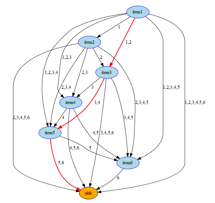 |
| Feasible solution for T=3 |
Selecting a link from item \(i\) to item \(j\) means: put items \(i,i+1,\dots,j-1\) into a box with size \(j-1\). Similarly, a link from item \(i\) to the sink node means: put items \(i,i+1,\dots,n\) into a box with size \(n\) (where \(n\) is the largest item or box).
The cost coefficients are defined by: \[\begin{align}c_{i,j} &= \mathit{size}_{j-1}^2 \sum_{k=i}^{j-1} \mathit{count}_k & \forall i\le j\\c_{i,\mathit{sink}} &= \mathit{size}_n^2 \sum_{k=i}^n \mathit{count}_k & \forall i \end{align}\]
We want to solve a shortest path problem from item 1 to the sink node with a side constraint: the number of "blue" nodes we visit should be exactly \(T\). The side constraint makes this a cardinality constrained or hop constrained shortest path problem. We can solve this as an MIP problem: \[\bbox[lightcyan,10px,border:3px solid darkblue] {\begin{align}min & \sum_{(i,j)\in A} c_{i,j} x_{i,j} \\ & \sum_{(j,i)\in A} x_{j,i} + b_i = y_i & \forall i & \>\> \text{(flow balance)}\\ & y_i = \sum_{(i,j)\in A} x_{i,j} & \forall i & \>\>\text{(outflow node $i$)}\\ &\sum_{i \ne \mathit{sink}} y_i = T &&\text{(cardinality)}\\ & x_{i,j},y_i \ge 0 \end{align} }\] Here \(b_i\) is the net exogenous supply of node \(i\). I.e. \[b_i = \begin{cases} 1 & \>\> \text{if $i=1$}\\ -1 & \>\> \text{if $i=\mathit{sink}$}\\ 0 & \>\>\text{otherwise}\end{cases}\]
----    470 VARIABLE cost.L                =  3.291991E+8

----    470 VARIABLE x.L  arcs

            i156        i269        i352        sink

i1         1.000
i156                   1.000
i269                               1.000
i352                                           1.000
This means our optimal grouping is \(i_1 - i_{155}\), \(i_{156} - i_{268}\), \(i_{269} - i_{351}\), \(i_{352} - i_{384}\). This is the same solution as for our set partitioning model.
GAMS Code
The GAMS code for this model can look like:
$ontext
Select Boxes Cardinality constrained shortest path $offtext sets iext 'orig nodes + sink' /i1*i384,sink/ i(iext) 'orig nodes w/o sink' /i1*i384/ ; table data(i,*) size count i1 156 1 i2 162 1 i3 168 1 i4 178 2 . . . i381 823 1 i382 827 2 i383 855 2 i384 864 1 ; parameter count(i), size(i); count(i) = data(i,'count'); size(i) = data(i,'size'); scalar T 'number of different box sizes' /4/; alias(iext,jext); alias(i,j,k); sets ij(i,j) 'allowed i,j combinations: i<=j' ijk(i,j,k) 'allowed i,j,k combinations: i<=k<=j' ; singleton set lastj(j) 'last element of j'; ij(i,j) = ord(i)<=ord(j); ijk(ij(i,j),k) = ord(k)>=ord(i) and ord(k)<=ord(j); lastj(j) = ord(j)=card(j); * * network topology * set a(iext,iext) 'arcs'; a(ij) = yes; a(i,'sink') = yes; parameter c(iext,iext) 'cost coefficients'; c(a(i,j)) = sqr(size(j-1)) * sum(ijk(i,j-1,k),count(k)); c(i,'sink') = sqr(size(lastj)) * sum(ijk(i,lastj,k),count(k)); parameter pinflow(iext) 'source/sink' / sink -1 i1 1 /; binary variables x(iext,iext) 'arcs' y(iext) 'outflow of node' ; variables cost; equations nodbal 'node balance' calcoutflow 'calc y' numboxes 'we need an active node for box' obj 'objective' ; obj.. cost =e= sum(a,c(a)*x(a)); calcoutflow(iext).. y(iext) =e= sum(a(iext,jext),x(a)); nodbal(iext).. sum(a(jext,iext), x(a)) + pinflow(iext) =e= y(iext); numboxes.. sum(i,y(i)) =e= T; model m /all/; * for this data set we can solve as LP (to be safe solve as MIP) solve m minimizing cost using rmip; display cost.l, x.l; * check if close to integer solution abort$sum((iext,jext)$(abs[x.l(iext,jext)-round(x.l(iext,jext))]>1e-4),1) "non-integer solution: solve as MIP"; * * reporting * set xij(i,jext) 'items i..j to into same box'; xij(i,jext) = x.l(i,jext+1) > 0.5; parameter results(*,*,*); results(xij(i,j),'minsize') = size(i); results(xij(i,j),'maxsize') = size(j); results(xij(i,j),'area') = sqr(size(j)); results(xij(i,j),'count') = sum(ijk(i,j,k),count(k)); results(xij(i,j),'sum area') = sqr(size(j)) * sum(ijk(i,j,k),count(k)); results('total','','sum area') = cost.l; results('total','','count') = sum(ijk(xij(i,j),k),count(k)); display results; |
Network Model II
The previous model was a network model with a side constraint. We can create a pure network by augmenting the network. Basically we keep track of the number of different boxes by indexing the nodes by item number and layer number. This means we have a larger number of nodes. The network can look like:
 |
| Layered network |
The results for the original data set with \(T=4\) looks like:
----    467 VARIABLE cost.L                =  3.291991E+8

----    467 VARIABLE x.L  arcs

            i156.layer2 i269.layer3 i352.layer4  sink.Lsink

i1  .layer1        1.00
i156.layer2                    1.00
i269.layer3                                1.00
i352.layer4                                            1.00
Note again that this must be interpreted as follows: group items \(i_1 - i_{155}\), \(i_{156} - i_{268}\), \(i_{269} - i_{351}\), \(i_{352} - i_{384}\) in box sizes large enough to hold \(i_{155}\), \(i_{268}\), \(i_{351}\), \(i_{384}\) . This is the same solution as for our earlier models.
GAMS Model
$ontext
Select Boxes Shortest path in layered network $offtext sets iext 'orig nodes + sink' /i1*i384,sink/ i(iext) 'orig nodes w/o sink' /i1*i384/ Lext 'orig layers + sink' /layer1*layer4,Lsink/ L(Lext) 'lyaers w/o sink' /layer1*layer4/ ; table data(i,*) size count i1 156 1 i2 162 1 i3 168 1 i4 178 2 . . . i381 823 1 i382 827 2 i383 855 2 i384 864 1 ; parameter count(i), size(i); count(i) = data(i,'count'); size(i) = data(i,'size'); scalar T 'number of different box sizes'; T = card(L); alias(iext,jext); alias(i,j,k); alias(Lext,L1ext,L2ext); alias(L,L1,L2); sets ij(i,j) 'allowed i,j combinations: i<=j' ijk(i,j,k) 'allowed i,j,k combinations: i<=k<=j' ; singleton sets lastj(j) 'last element of j' lastL(L) 'last element of L' ; ij(i,j) = ord(i)<=ord(j); ijk(ij(i,j),k) = ord(k)>=ord(i) and ord(k)<=ord(j); lastj(j) = ord(j)=card(j); lastL(L) = ord(L)=card(L); * * network topology * set a(iext,L1ext,jext,L2ext) 'arcs'; a(i,L1,j,L1+1) = ord(j)>ord(i); a(i,lastL,'sink','Lsink') = yes; parameter c(iext,L1ext,jext,L2ext) 'cost coefficients'; c(a(i,L1,j,L2)) = sqr(size(j-1)) * sum(ijk(i,j-1,k),count(k)); c(i,lastL,'sink','Lsink') = sqr(size(lastj)) * sum(ijk(i,lastj,k),count(k)); parameter pinflow(iext,Lext) 'source/sink' / sink.Lsink -1 i1.layer1 1 /; binary variables x(iext,Lext,iext,Lext) 'arcs' ; variables cost; equations nodbal 'node balance' obj 'objective' ; obj.. cost =e= sum(a,c(a)*x(a)); nodbal(iext,L1ext).. sum(a(jext,L2ext,iext,L1ext), x(a)) + pinflow(iext,L1ext) =e= sum(a(iext,L1ext,jext,L2ext), x(a)); model m /all/; * this is a pure network: we can solve as an LP solve m minimizing cost using rmip; option x:2:2:2; display cost.l, x.l; * * reporting * set xij(i,jext) 'items i..j to into same box'; xij(i,jext) = sum((L1ext,L2ext),x.l(i,L1ext,jext+1,L2ext)) > 0.5; parameter results(*,*,*); results(xij(i,j),'minsize') = size(i); results(xij(i,j),'maxsize') = size(j); results(xij(i,j),'area') = sqr(size(j)); results(xij(i,j),'count') = sum(ijk(i,j,k),count(k)); results(xij(i,j),'sum area') = sqr(size(j)) * sum(ijk(i,j,k),count(k)); results('total','','sum area') = cost.l; results('total','','count') = sum(ijk(xij(i,j),k),count(k)); display results; |
As this is a pure network, we can ask Cplex to use the network simplex method to solve this. We see:
---   1,537 rows  220,993 columns  662,977 non-zeroes
---   220,992 discrete-columns
--- Executing CPLEX: elapsed 0:01:15.411

...

Tried aggregator 1 time.
LP Presolve eliminated 393 rows and 219470 columns.
Aggregator did 764 substitutions.
Reduced LP has 380 rows, 759 columns, and 1138 nonzeros.
Presolve time = 2.25 sec. (568.28 ticks)
Extracted network with 381 nodes and 759 arcs.
Extraction time = 0.00 sec. (0.11 ticks)

Iteration log . . .
Iteration:     0   Infeasibility     =             1.000000 (24337)
Iteration:   100   Infeasibility     =             1.000000 (24337)
Iteration:   200   Infeasibility     =             1.000000 (24337)

Network - Optimal:  Objective =    3.2919911900e+08
Network time = 0.00 sec. (0.07 ticks)  Iterations = 261 (261)
LP status(1): optimal
Cplex Time: 2.39sec (det. 588.24 ticks)
We see the presolver takes most of the time, but is also highly effective. The presolved model takes zero seconds to solve.
Dynamic Programming
A dynamic programming algorithm is an alternative for this problem. If we define \[f_{i,b} = \text{minimum total area when we pack items $1,\dots,i$ (ordered and with unique size) in $b$ box sizes}\] then we can write down the recursion:\[ f_{i,b} = \min_{k=b-1,\dots,i-1} \left\{ f_{k,b-1} + \mathit{size}_i^2 \sum_{j=k+1}^i \mathit{count}_j \right\}\]
When we code this up in R we could see something like:
data <- c(
  156,162,168,178,178,180,185,185,190,192,193,194,195,195,197,197,198,198,199,200,202,206,
  206,210,210,210,212,212,214,215,217,217,217,217,217,218,220,220,220,220,220,220,220,220,
  ...
  727,730,733,733,734,734,734,735,735,735,738,740,743,744,754,755,755,755,755,755,758,760,
  766,766,780,780,780,780,780,780,780,782,783,785,795,805,806,820,823,827,827,855,855,864)

t<-table(data)
count <- as.vector(t)
size <- as.numeric(rownames(t))

cumulative <- cumsum(count)

# number of box sizes, number of item sizes
NB <- 4
NI <- length(size)

# allocate matrix NI rows, NB columns (initialize with NAs)
# f[ni,nb] = cost when we have ni items and nb blocks
F <- matrix(NA,NI,NB)
S <- matrix("",NI,NB)

# initialize for nb=1
F[1:NI,1] <- cumulative * size[1:NI]^2
S[1:NI,1] <- paste("(",1,"-",1:NI,")",sep="")

# dyn programming loop
for (nb in 2:NB) {
  for (ni in nb:NI) {
     k <- (nb-1):(ni-1)
     v <- F[k,nb-1] + (cumulative[ni]-cumulative[k])*size[ni]^2
     F[ni,nb] <- min(v)

     # create path (string)
     mink <- which.min(v) + nb - 2
     s <- paste("(",mink+1,"-",ni,")",sep="")
     S[ni,nb] <- paste(S[mink,nb-1],s,sep=",")
  }
}

for (nb in 1:NB) {
   cat(sprintf("%s boxes: %s, total area = %g\n",nb,S[NI,nb],F[NI,nb]))
}
Note that the inner \(k\) loop is vectorized. The results look like:
1 boxes: (1-384), total area = 8.70414e+08
2 boxes: (1-268),(269-384), total area = 4.59274e+08
3 boxes: (1-155),(156-284),(285-384), total area = 3.66837e+08
4 boxes: (1-155),(156-268),(269-351),(352-384), total area = 3.29199e+08
The results for 1,2 and 3 boxes we get for free.
Data
The data set used here is shown below:
  156,162,168,178,178,180,185,185,190,192,193,194,195,195,197,197,198,198,199,200,202,206
  206,210,210,210,212,212,214,215,217,217,217,217,217,218,220,220,220,220,220,220,220,220
  220,220,222,223,223,224,225,225,225,225,225,225,225,226,226,226,227,228,228,228,228,230
  230,230,230,230,230,230,230,230,230,230,230,230,232,232,232,233,233,234,234,235,235,235
  235,238,238,238,238,240,240,240,240,240,240,240,240,240,241,242,242,242,242,243,244,244
  244,245,246,247,247,247,249,250,250,250,250,250,251,252,252,252,252,253,254,254,254,255
  255,255,255,255,256,256,257,257,257,258,258,258,258,258,259,260,260,260,260,260,260,260
  260,260,262,262,262,262,262,262,262,264,264,264,265,265,265,265,265,266,267,267,267,267
  268,268,268,268,268,268,269,270,270,270,270,270,270,270,270,270,270,271,272,272,272,272
  272,273,273,273,273,274,274,274,274,274,275,275,275,275,275,275,277,277,277,278,278,278
  278,278,278,280,280,280,280,281,282,282,284,285,285,285,285,285,285,287,287,287,288,288
  288,288,288,289,290,290,290,290,290,290,290,290,290,290,290,292,292,293,293,294,294,294
  295,295,295,295,295,295,295,295,296,296,297,297,298,298,298,298,300,300,300,300,300,300
  300,300,300,300,300,300,300,300,302,302,303,303,303,303,304,305,305,305,305,305,306,306
  307,308,308,308,310,310,310,310,310,310,310,312,312,312,312,313,315,315,315,315,315,315
  315,315,315,317,317,317,317,318,318,318,318,320,320,320,320,320,320,320,320,320,320,320
  320,320,322,323,323,325,325,325,325,326,326,327,327,328,328,330,330,330,330,330,330,330
  332,333,333,334,334,334,334,335,335,335,335,335,336,336,336,338,338,339,339,340,340,340
  340,340,340,340,342,342,342,342,343,345,345,345,345,345,345,345,346,346,346,347,347,348
  348,348,349,350,350,350,350,350,350,350,350,350,350,350,350,350,350,350,350,350,350,352
  352,353,353,353,353,354,354,354,356,357,357,357,357,358,358,360,360,360,360,360,360,360
  360,360,360,360,360,361,362,362,362,363,363,364,364,364,364,365,365,365,365,365,365,365
  367,367,367,368,370,370,370,370,370,370,370,370,370,372,372,372,373,375,375,375,375,375
  375,377,377,377,378,380,380,380,380,380,380,380,380,380,380,380,380,381,382,383,383,383
  383,384,384,384,384,385,385,385,386,386,386,386,387,387,387,387,388,388,388,388,388,389
  390,392,392,393,394,394,395,396,397,397,398,398,398,400,400,400,400,400,400,400,400,405
  405,408,410,410,410,410,410,410,412,412,412,412,412,413,415,415,416,416,417,417,418,418
  419,419,419,420,420,420,420,420,420,420,420,423,423,423,423,424,424,425,425,425,428,428
  430,430,430,430,430,430,430,430,430,430,430,430,431,432,432,432,432,433,433,433,433,433
  434,434,435,435,435,435,437,438,438,438,438,440,440,440,440,440,440,440,441,442,443,444
  444,445,445,445,445,445,445,445,445,446,447,448,448,450,450,450,450,450,450,450,450,450
  452,453,453,455,455,455,455,456,457,458,458,458,458,459,460,460,460,460,460,460,460,462
  462,463,464,465,465,465,465,465,465,465,466,466,467,467,467,467,467,468,468,468,469,469
  470,470,470,470,470,470,470,470,470,472,472,472,474,475,475,476,478,478,478,478,480,480
  480,480,480,480,480,480,480,480,480,480,482,482,482,482,482,482,482,485,485,485,485,488
  488,488,488,490,490,490,490,490,490,490,490,491,491,492,492,492,492,492,492,492,493,493
  495,495,495,496,497,498,498,498,498,498,498,498,499,500,500,500,500,500,500,502,502,502
  505,505,505,505,505,506,507,507,510,510,510,510,510,510,510,510,510,510,510,510,512,512
  513,514,515,515,517,517,518,520,520,520,520,520,520,522,523,523,523,524,525,525,525,525
  525,525,528,528,528,528,528,528,528,530,530,530,530,530,530,531,532,534,535,535,535,535
  535,536,538,538,538,539,540,540,540,540,540,540,540,540,540,540,540,541,543,543,543,544
  544,545,545,545,546,546,546,547,547,548,548,550,550,550,550,550,550,550,550,550,550,550
  550,550,552,552,555,555,555,555,555,555,555,557,557,557,557,560,560,560,560,560,562,562
  563,563,564,565,565,565,565,565,565,567,567,568,568,569,569,569,570,570,570,571,572,572
  573,574,574,574,576,576,578,580,580,580,584,585,585,587,588,590,592,593,596,597,600,600
  600,600,602,602,602,602,602,603,604,605,605,605,605,605,605,605,607,607,607,608,610,610
  610,610,610,610,612,612,612,612,615,615,615,615,618,618,620,622,624,625,625,625,627,627
  628,628,628,630,630,632,633,635,635,637,638,638,640,640,640,640,640,642,643,647,648,649
  650,650,655,655,655,656,660,660,660,660,660,662,662,663,664,664,664,664,665,665,665,670
  670,672,677,677,679,680,680,680,680,680,685,685,687,688,690,690,692,694,695,697,698,700
  700,701,704,704,705,705,705,705,705,705,705,705,705,710,710,712,715,717,720,720,722,723
  727,730,733,733,734,734,734,735,735,735,738,740,743,744,754,755,755,755,755,755,758,760
  766,766,780,780,780,780,780,780,780,782,783,785,795,805,806,820,823,827,827,855,855,864
References
- Need to create 3−4 different box sizes and to minimize material waste for a set of n objects that need to fit into these boxes, https://math.stackexchange.com/questions/2843990/need-to-create-3-4-different-box-sizes-and-to-minimize-material-waste-for-a-se/2850260
- On the scheduling of reading book chapters, https://yetanothermathprogrammingconsultant.blogspot.com/2018/02/on-scheduling-of-reading-book-chapters.html
No comments:
Post a Comment