Saturday, December 31, 2016

Smart Slime Mold on page 3 of the Washington Post

image

References

  1. Washington Post article: https://www.washingtonpost.com/news/speaking-of-science/wp/2016/12/30/the-strange-case-of-the-slime-molds-that-can-learn-and-teach-one-another
  2. Slime mold and linear programming: http://yetanothermathprogrammingconsultant.blogspot.com/2016/02/slime-mold-and-linear-programming.html

MIP Modeling

In an investment planning model I needed to model the following:

image

We can build a facility during any time period. So we have:

\[\begin{align}&build_t \in \{0,1\} \\
                   &\sum_t build_t \le 1\end{align}\]

The variable \(open_t\in \{0,1\}\) indicates we have an open facility, ready to do business. A facility is considered open after it is built (we don’t close facilities during the planning horizon). To be more precise: it becomes available one period after it has been built.

There are actually a few ways to model this:

alternative 1

Look if the facility was built in any period \(t’<t\):

\[open_t = \sum_{t’|t’<t} build_{t’}\]
alternative 2

Use an ‘or’ formulation:

\[open_t = build_{t-1} \textbf{ or } open_{t-1}\]

This can be linearized as:

\[\begin{align}&open_t \ge build_{t-1}\\
                    &open_t \ge open_{t-1}\\
                    &open_t \le build_{t-1}+open_{t-1}\end{align}\]

alternative 3

We can simplify the recursive construct:

\[open_t = build_{t-1}+open_{t-1}\]

With this, we now explicitly forbid \(build_{t-1}+open_{t-1}=2\) which was not allowed (implicitly) anyway.

The last formulation seems preferable in terms of simplicity and the number of non-zero elements needed.

As usual with lags we need to be careful what happens near the borders, in this case when \(t=t1\). We just can fix \(open_{t1}=0\). When using GAMS you can even skip that, as indexing with lags outside the domain returns zero. Here that means \(open_{t1} = build_{t1-1} + open_{t1-1} = 0 + 0\). We can also verify this in the equation listing:

---- eqopen2  =E= 

eqopen2(t1)..  open(t1) =E= 0 ; (LHS = 0)
    
eqopen2(t2)..  - build(t1) - open(t1) + open(t2) =E= 0 ; (LHS = 0)
    
eqopen2(t3)..  - build(t2) - open(t2) + open(t3) =E= 0 ; (LHS = 0)
    
REMAINING 3 ENTRIES SKIPPED

Wednesday, December 28, 2016

Unique Solutions in KenKen

In (1) a MIP model is proposed so solve the KenKen puzzle. During a discussion, the question came up if I could prove the uniqueness of a solution. In the Mixed Integer Programming model I used a standard formulation for a solution: 

\[x_{i,j,k} = \begin{cases}1 & \text{if cell $(i,j)$ has the value $k$}\\
                                    0 & \text{otherwise}\end{cases}\]

A general approach could be to use the technique described in (2): add a cut to forbid the current solution and solve again. If this second solve is infeasible we have established that the original solution was unique.

In this case we can use a more specialized cut that is simpler:

\[\sum_{i,j,k} x^*_{i,j,k} x_{i,j,k} \le n^2-1\]

where \(x^*\) is the previous solution and \(n \times n\) is the size of the puzzle.

To test this with the model and problem data shown in (1) I used:

image

Note that \(\displaystyle\sum_{i,j,k|x^*_{i,j,k}=1} x_{i,j,k}\) is identical to \(\displaystyle\sum_{i,j,k} x^*_{i,j,k} x_{i,j,k}\). To make sure things work correctly with solution values like 0.9999, I actually used a somewhat generous tolerance: \(\displaystyle\sum_{i,j,k|x^*_{i,j,k}>0.5} x_{i,j,k}\).

Indeed the solution from the first solve was unique. The second solve yielded:

               S O L V E      S U M M A R Y

     MODEL   kenken2             OBJECTIVE  z
     TYPE    MIP                 DIRECTION  MINIMIZE
     SOLVER  CPLEX               FROM LINE  115

**** SOLVER STATUS     1 Normal Completion        
**** MODEL STATUS      10 Integer Infeasible      
**** OBJECTIVE VALUE               NA

RESOURCE USAGE, LIMIT          0.031      1000.000
ITERATION COUNT, LIMIT         0    2000000000

This approach can also be applied to the Sudoku MIP model.

References
  1. KenKen puzzle solved using a MIP model: http://yetanothermathprogrammingconsultant.blogspot.com/2016/10/mip-modeling-from-sudoku-to-kenken.html
  2. Forbid a given 0-1 solution: http://yetanothermathprogrammingconsultant.blogspot.com/2011/10/integer-cuts.html

Tuesday, December 20, 2016

SAS/OR MIP solver

In (1) the performance of the SAS/OR MIP solver is discussed. It uses the MIPLIB problem set. Timings from different studies are always difficult to compare, but if we take the 214 or 218 feasible problems, and measure how many of those problems could be solved within in 2 hours we see:

Solver Number solved within 2 hours (12 threads) Source
CBC 119 of 218 (3)
SAS/OR 170 of 214 (1)
Cplex 204 of 218 (3)
Gurobi 210 of 218 (3)

I think it is fair to guess that the SAS solver is faster than CBC but a little bit slower than the market leaders Cplex and Gurobi. Again: I don’t know the difference in speed between the machines these benchmarks were executed on, so take this with a grain of salt.

I have quite a few clients with large SAS licenses, but they typically do not use SAS/OR. As a result I have never used the SAS/OR solvers. I usually use SAS as a database. My typical workflow is: export the SAS data, combine with other data, develop and solve the models with other tools and report solutions in Excel.

References
  1. Imre PĆ³lik, How good is the MILP solver in SAS/OR?, December 2016, http://blogs.sas.com/content/operations/2016/12/19/good-milp-solver-in-sasor/
  2. Philipp M. Christophel e.a., The SAS MILP Solver: Current Status and Future Development, INFORMS 2016 meeting, http://blogs.sas.com/content/operations/files/2016/12/Christophel_INFORMS2016.pdf 
  3. H. Mittelmann, The solvable MIPLIB instances (MIPLIB2010), http://plato.asu.edu/ftp/solvable.html

Sunday, December 18, 2016

MonetDB and R

logo

MonetDB (1) is a so-called column-oriented database or column-store (2). It is server based, SQL compliant and open-source. The column orientation can lead to better performance for certain types of tasks, especially OLAP and ETL (i.e. analytical work). Traditional row-wise databases are said to be more appropriate for OLTP workloads.  

MonetDBLite

There exists a CRAN package to let R talk to a MonetDB server (MonetDB.R). There is also a different package called MonetDBLite. This contains an in-process version of MonetDB.  This means MonetDBLite is more or less an alternative for RSQLite (4). A picture comparing the performance of MonetDBLite is from (4):

Basically the more towards the left-lower corner the better.

In (3) there are some timings comparing MonetDBLite to SQLite. E.g. converting a (large) table to a data frame:

There is lots of data traffic from the database to R and the server based MonetDB.R does not finish the larger tables (traffic has to go through a TCP/IP socket). But the embedded database is very fast compared to SQLite.

This looks like an interesting database for R related work.

References
  1. MonetDB The column-store pioneer, https://www.monetdb.org/Home
  2. Daniel Adabi, Distinguishing Two Major Types of Column-Stores, March 2010, http://dbmsmusings.blogspot.com/2010/03/distinguishing-two-major-types-of_29.html
  3. https://www.monetdb.org/blog/monetdblite-r
  4. Anthony Damico, MonetDBLite because fast, June 2016,  https://www.r-bloggers.com/monetdblite-because-fast/
  5. Using MonetDB[Lite] with real-world CSV files, https://www.r-bloggers.com/using-monetdblite-with-real-world-csv-files/

Saturday, December 17, 2016

New book: Optimization by GRASP; Greedy Randomized Adaptive Search Procedures

This is a well known meta-heuristic (with a somewhat less flashy name than some of the new heuristics that get invented every week). Apparently this is the first book fully dedicated to GRASP. GRASP was introduced in 1989 by Feo and Resende (2).

Chapters:
  1. Introduction
  2. A short tour of combinatorial optimization and computational complexity
  3. Solution construction and greedy algorithms
  4. Local search
  5. GRASP: The basic heuristic
  6. Runtime distributions
  7. Extended construction heuristics
  8. Path-relinking
  9. GRASP with path-relinking
  10. Parallel GRASP heuristics
  11. GRASP for continuous optimization
  12. Case studies

References
  1. Mauricio G. C. Resende and Celso C. Ribiero, Optimization by GRASP,  Springer 2016. Price: about $0.25 per page (some of them with color pictures).
  2. T.A. Feo and M.G.C. Resende, A probabilistic heuristic for a computationally difficult set covering problem, Operations Research Letters, 8:67–71, 1989.

Tuesday, December 13, 2016

Multiple solutions in stylized flood planning model

flood-965092_640

For a project I was looking at a simple two stage stochastic integer programming problem (1).

I find it always very rewarding to reproduce the results in  the paper. Re-implementing the model forces me to not skip the details. Compared to superficial reading it requires to pay attention to all aspects. Of course in many cases journal papers do not allow to reproduce results because crucial details or data are left out. Presenting a stylized model illustrating and illuminating the concepts is only done sporadically, may be because it is actually hard to create such a “simple” model, and it may look less “scientific”.

The model is a fairly standard 2 stage SLP. In stage 1 we can implement so-called permanent floodplain management actions (raising structures, implement warning systems, etc.) The realizations are floods of different sizes. In stage 2 we can apply certain emergency measures (evacuations, issue sandbags etc.).

After re-implementing the model I saw the same objective function values, but the stage 2 variables differed a bit.

The paper shows a table with the stage 2 results:

image

In GAMS we do not see any of the levee monitoring being implemented:

----    145 VARIABLE xe.L  stage 2 decisions: emergency options

             peak5-6     peak6-8    peak8-10     peak10+

evacuate                   1.000       1.000       1.000
sandbag        2.000       2.000

GAMS will report marginals (duals and reduced costs) even for a MIP. They fix the integer variables and resolve as an LP to get these. Here are the relevant marginals:

----    145 VARIABLE xe.M  stage 2 decisions: emergency options

             peak0-5     peak5-6     peak6-8    peak8-10     peak10+

evacuate   80000.000    7900.000  -12000.000   -8000.000   -9000.000
sandbag    24000.000  -12200.000  -46200.000     600.000     300.000
monitor        0.800       0.079         EPS       0.020       0.010

This EPS means this variable is non-basic with a zero reduced cost. This can indicate the presence of multiple optima. Indeed when using a different MIP solver I see:

----    145 VARIABLE xe.L  stage 2 decisions: emergency options

             peak5-6     peak6-8    peak8-10     peak10+

evacuate                   1.000       1.000       1.000
sandbag        2.000       2.000
monitor                20000.000

which is the same as the results in the paper.

Digging a little bit further, we can see that the damage reduction by implementing emergency measure “monitor” is the same as its cost. This means we are indifferent whether to apply this option in this scenario.

----    154 PARAMETER red2  damage reduction b(j,s)*xe.l(j,s)

             peak5-6     peak6-8    peak8-10     peak10+

evacuate              300000.000  500000.000 1000000.000
sandbag  2000000.000 1600000.000
monitor                20000.000


----    154 PARAMETER c2  emergency option cost ce(j)*xe.l(j,s)

             peak5-6     peak6-8    peak8-10     peak10+

evacuate              100000.000  100000.000  100000.000
sandbag    60000.000   60000.000
monitor                20000.000

I would guess the chance this will happen with real data is smaller than with these nicely rounded invented data.

The model itself is implemented as a fairly standard deterministic equivalent formulation:

image

References
  1. Jay R. Lund, Floodplain Planning with Risk-based Optimization, Journal of Water Resources Planning and Management, Vol. 127, No. 3, May 2002

PyMathProg: another Python based modeling tool

Project homepage: http://pymprog.sourceforge.net/

Uses GLPK as solver. Here is a small example:

from pymprog import * 
c = (10, 6, 4)
A = [ ( 1, 1, 1),     
      ( 9, 4, 5),   
      ( 2, 2, 6) ]   
b = (10, 60, 30)
begin('basic') # begin modelling
verbose(True)  # be verbose
x = var('x', 3) #create 3 variables
maximize(sum(c[i]*x[i] for i in range(3)))
for i in range(3):
  sum(A[i][j]*x[j] for j in range(3)) <= b[i] 
solve() # solve the model
sensitivity() # sensitivity report
end() #Good habit: do away with the model

There is quite some competition in this space. Some of the major competitors:

Saturday, December 10, 2016

Sorting inside a MIP model

This does not happen a lot, but in some cases we want to sort decision variables. This turns out not such an easy exercise.

When not to use sorting

If we deal with just the \(\min()\) or \(\max()\) function we can do things better than sorting. An important trick is to exploit any so-called convexity so we don’t need to add extra binary variables. Even if the problem is not convex, there is no need to sort things.

Interestingly, minimizing the sum of the K largest values also does not need sorting. See (4).

Sorting a parameter

At first sight this is not very useful exercise: we can sort a parameter – constants in the model – outside of the model. However the problem demonstrates some of the concepts I will use later on. Assume \(a_j\) is our given parameter. A permutation \(y\) of \(a\) can be written as \(y=Pa\) where \(P\) is a permutation matrix (1). A permutation matrix is an identity matrix \(I\) with rows and columns interchanged. Such a matrix has exactly a 1 in each row and in each column. A different way to look at this is as an assignment problem with binary variables \(p_{i,j} \in \{0,1\}\).

The linear constraints to sort \(a_j\) (descending) can look like:

\[\boxed{\begin{align}
&\sum_i p_{i,j} = 1 \>\> \forall j\\
&\sum_j p_{i,j} = 1 \>\> \forall i\\
&y_i = \sum_j p_{i,j} a_j \\
&y_i \ge y_{i+1} \\
&p_{i,j} \in \{0,1\}
\end{align}}\]

Here indices \(i\) and \(j\) are from sets with the same cardinality (\(n\)), i.e. \(p_{i,j}\) is a square matrix. Note that we use \(n^2\) binary variables here, so don’t expect this to work for very large vectors \(a_j\) (2). The same structure can also be used in the context of all-different constraints (3).

Example results

----     32 PARAMETER a 

j1 2,    j2 4,    j3 1,    j4 3


----     32 VARIABLE p.L 

            j1          j2          j3          j4

i1                       1
i2                                               1
i3           1
i4                                   1


----     32 VARIABLE y.L 

i1 4,    i2 3,    i3 2,    i4 1

Sorting a variable

Instead of sorting a parameter \(a_j\), consider the problem of sorting a variable \(x_j\). We cannot just replace \(a_j\) by \(x_j\) as

\[y_i = \sum_j p_{i,j} x_j \]

is non-linear. There is a way to linearize the product \(q_{i,j} = p_{i,j} x_j\) as this is a multiplication of a binary variable with a continuous variable. Assuming \(x_j \in [0,U_j]\), we have:

\[\begin{align}
&0\le q_{i,j} \le U_j p_{i,j}\\
&x_j – U_j (1-p_{i,j}) \le q_{i,j} \le x_j
\end{align}\]
Example results

----     41 VARIABLE x.L 

j1 0.172,    j2 0.843,    j3 0.550,    j4 0.301


----     41 VARIABLE p.L 

            j1          j2          j3          j4

i1                       1
i2                                   1
i3                                               1
i4           1


----     41 VARIABLE q.L 

            j1          j2          j3          j4

i1                   0.843
i2                               0.550
i3                                           0.301
i4       0.172


----     41 VARIABLE y.L 

i1 0.843,    i2 0.550,    i3 0.301,    i4 0.172

A different formulation

A different way to formulate a sorting scheme is to look at the problem as a special transportation problem. Transportation equations look like:

\[\boxed{\begin{align}
&\sum_i z_{i,j} = x_j \>\> \forall j\\
&\sum_j z_{i,j} = y_i \>\> \forall i
\end{align}}\]

As can be seen this is linear in \(x\). We still need to enforce that one supply node is linked to exactly one demand node. This can be done using an additional assignment block:

\[\boxed{\begin{align}
&\sum_i p_{i,j} = 1 \>\> \forall j\\
&\sum_j p_{i,j} = 1 \>\> \forall i\\
&\sum_i z_{i,j} = x_j \>\> \forall j\\
&\sum_j z_{i,j} = y_i \>\> \forall i\\
&y_i \ge y_{i+1} \\
&0\le z_{i,j} \le p_{i,j} U_j\\
&p_{i,j} \in \{0,1\}
\end{align}}\] 
Example results

----     43 VARIABLE x.L 

j1 0.172,    j2 0.843,    j3 0.550,    j4 0.301


----     43 VARIABLE p.L 

            j1          j2          j3          j4

i1                       1
i2                                   1
i3                                               1
i4           1


----     43 VARIABLE z.L 

            j1          j2          j3          j4

i1                   0.843
i2                               0.550
i3                                           0.301
i4       0.172


----     43 VARIABLE y.L 

i1 0.843,    i2 0.550,    i3 0.301,    i4 0.172

Example

From this post:

I'm currently stuck with a MIP program where the interest rate, i, is based on the number of units produced for Housing Plan A. If the number of plan A houses sold is the highest among all four types then i=1. If the number of plan A houses sold is the second highest, then i=2 and so on up to i=4. The interest rate is basically 2i%. Not really sure how to add constraints that will represent the position of plan A houses and implement the correct interest rate in the objective function. The objective function maximizes the total profit (e.g 50,000A + 40,000B + 70,000C + 80,000D). Any ideas on how to use binary variables to represent position?

image

image

Some results can look like:

----     47 VARIABLE x.L 

A 100.000,    B  90.000,    C 120.000,    D 150.000


----     47 VARIABLE p.L  permutation matrix

            1           2           3           4

A                               1.000
B                                           1.000
C                   1.000
D       1.000


----     47 VARIABLE q.L  p(i,j)*x(i)

            1           2           3           4

A                             100.000
B                                          90.000
C                 120.000
D     150.000


----     47 VARIABLE xsorted.L 

1 150.000,    2 120.000,    3 100.000,    4  90.000


----     47 VARIABLE r.L 

A 0.060,    B 0.080,    C 0.040,    D 0.020

References
  1. Permutation Matrix, https://en.wikipedia.org/wiki/Permutation_matrix
  2. Sorting by MIP, http://yetanothermathprogrammingconsultant.blogspot.com/2011/10/sorting-by-mip.html, about sorting a parameter
  3. All-different and Mixed Integer Programming, http://yetanothermathprogrammingconsultant.blogspot.com/2016/05/all-different-and-mixed-integer.html
  4. Paul Rubin, Optimizing Part of the Objective II, http://orinanobworld.blogspot.com/2015/08/optimizingpartoftheobjectivefunction-ii.html

Friday, December 9, 2016

Reading CSV files in R: read.csv vs read_csv

There are a number of very fast CSV file readers available in R and Python. Lets have a quick test to see how they compare.

Generating CSV file

I generated a very simple, but large CSV file with 100 million records using a GAMS script as follows:

set
  i
/a1*a100/
  j
/b1*b100/
  k
/c1*c100/
  l
/d1*d100/
;

parameter d(i,j,k,l);
d(i,j,k,l) = uniform(0,1);

$setenv gdxcompress 1
execute_unload "d.gdx"
,d;
execute "gdxdump d.gdx output=d.csv symb=d delim=comma format=csv"
;

The generated CSV file looks like:

D:\tmp\csv>head d.csv
"i","j","k","l","Val"
"a1","b1","c1","d1",0.171747132
"a1","b1","c1","d2",0.843266708
"a1","b1","c1","d3",0.550375356
"a1","b1","c1","d4",0.301137904
"a1","b1","c1","d5",0.292212117
"a1","b1","c1","d6",0.224052867
"a1","b1","c1","d7",0.349830504
"a1","b1","c1","d8",0.856270347
"a1","b1","c1","d9",0.067113723

D:\tmp\csv>dir d.*
Volume in drive D is My Passport
Volume Serial Number is 74B7-6DCC

Directory of D:\tmp\csv

12/08/2016  03:42 PM     3,656,869,678 d.csv
12/08/2016  03:30 PM       806,199,476 d.gdx
               2 File(s)  4,463,069,154 bytes
               0 Dir(s)  1,099,214,491,648 bytes free

D:\tmp\csv>

We also see the CSV file is much larger than the intermediate (compressed) GAMS GDX file.

R read.csv

This is the default CSV reader in R.

> system.time(d<-read.csv("d.csv"))
   user  system elapsed 
1361.61   50.56 1434.39 

R read_csv

read_csv is from the readr package, and it is much faster for large CSV files:

> system.time(d<-read_csv("d.csv"))
Parsed with column specification:
cols(
  i = col_character(),
  j = col_character(),
  k = col_character(),
  l = col_character(),
  Val = col_double()
)
|================================================================================| 100% 3487 MB
   user  system elapsed 
 186.23    5.66  196.20 

Would it help to read a compressed CSV file?

> system.time(d<-read_csv("d2.csv.gz"))
Error in .Call("readr_read_connection_", PACKAGE = "readr", con, chunk_size) : 
  negative length vectors are not allowed
Timing stopped at: 57.53 4.43 62.29 

Bummer. I have no idea what went wrong here. May be we hit some size limit (note the CSV file is larger than 2 gb; other compression formats gave the same result).

R fread

As mentioned in the comments, the package data.table has a function fread.

> system.time(dt<-fread("d.csv"))
Read 100000000 rows and 5 (of 5) columns from 3.406 GB file in 00:04:40
   user  system elapsed 
 275.19    4.33  281.05 
Python pandas.read_csv

Quite fast:

t0=pc()
df=pd.read_csv("d.csv")
print(pc()-t0)
158.2270488541103

The paratext library should be even faster.

References
  1. readr 1.0.0, https://blog.rstudio.org/2016/08/05/readr-1-0-0/
  2. Damian Eads, ParaText: CSV parsing at 2.5 GB per second, http://www.wise.io/tech/paratext

Thursday, December 8, 2016

Management Science on Vox

Fuel is cheap. Why are we still paying to check bags?


References
  1. Mariana Nicolae and Mazhar Arıkan and Vinayak Deshpande and Mark Ferguson, Do Bags Fly Free? An Empirical Analysis of the Operational Implications of Airline Baggage Fees, Management Science, August 2016 (online), http://dx.doi.org/10.1287/mnsc.2016.2500 

Tuesday, December 6, 2016

[VIDEO] A Huge Debate: R vs. Python for Data Science


Interesting video: [Video] A Huge Debate: R vs. Python for Data Science (presentation by Eduardo AriƱo de la Rubia)

Packages discussed:

image

R

Friday, December 2, 2016

Cplex 12.7 and Benders Decomposition

The new version of Cplex (12.7) has some interesting new facilities to make it easier to use a Benders Decomposition approach (1,3). Paul Rubin shares some experiences with this in (2).

image

The original paper by Jacques Benders can be found in (4). These old papers are always an interesting read. The style and notation is often very different from how papers look like these days, although in this case the notation is quite modern.

References
  1. Paul Shaw, What’s new in Cplex 12.7?, https://developer.ibm.com/docloud/blog/2016/11/11/whats-in-cos-12-7/
  2. Paul Rubin, Support for Benders Decomposition in CPLEXhttp://orinanobworld.blogspot.com/2016/12/support-for-benders-decomposition-in.html
  3. Xavier Nodet, IBM CPLEX Optimization Studio 12.7 - Benders, Modeling Assistance, etc., http://www.slideshare.net/xnodet/ibm-cplex-optimization-studio-127-benders-modeling-assistance-etc
  4. J.F. Benders, Partitioning procedures for solving mixed-variables programming problems, Numerische Mathematik 4, pp. 238-252, 1962, http://www.digizeitschriften.de/dms/img/?PID=GDZPPN001164228

Thursday, December 1, 2016

Table Assignment for Kindergartners

From this post we have a problem stated as:

My wife teaches AM and PM kindergarten classes. AM has 14 students and PM 11. At the beginning of each month, she puts out a new seating chart where she rotates students in such a way that they (ideally) sit at a different table and with different students for that month.

There are 3 students per table, but if numbers force the issue, the last may have more or less. We realize that, by the end of the year, there will be some unavoidable situations where students end up sitting with each other or at the same tables again, and this is okay.

Something like this I imagine:

2885861465_8b4101648a_z
Source

A somewhat related problem is discussed in (1). As usual we have a set of binary variables that indicate the assignment of students to tables: 

\[x_{s,t,m} = \begin{cases}1&\text{if student $s$ is seated at table $t$ in month $m$}\\
                                      0&\text{otherwise}\end{cases}\]

The first set of equations are somewhat straightforward. Each student sits at exactly one table:

\[\sum_t x_{s,t,m} = 1 \>\>\forall s,m\]

We cannot exceed the capacity of a table:

\[\sum_s x_{s,t,m} \le cap_t \>\> \forall t,m\]

In the complete model below I used an equality constraint for this: there is no slack capacity. Secondly we want to keep track of how many times students sit at the same table. We introduce binary variables \(meet_{s1,s2,t,m}\in\{0,1\}\) indicating if two students \(s1\) and \(s2\) sit at the same table. The obvious nonlinear equation would be:

\[meet_{s1,s2,t,m} = x_{s1,t,m} \cdot x_{s2,t,m}\>\> \forall s1<s2,t,m\]

Note that we can exploit symmetry here: if we already compared \(s1,s2\) we do not need to bother about \(s2,s1\). The standard linearization is

\[\begin{align} & meet_{s1,s2,t,m} \le x_{s1,t,m}\\
& meet_{s1,s2,t,m} \le x_{s2,t,m}\\
& meet_{s1,s2,t,m} \ge x_{s1,t,m}+x_{s1,t,m}-1\end{align}\]

As we push variable \(meet\) down, we can drop the first two inequalities and just keep the last. Note that variable \(meet\) is now a bound instead of the product \(x_{s1,t,m} \cdot x_{s2,t,m}\). When reporting we should use the underlying variables \(x\).

A count of the number of times students \(s1,s2\) sit at the same table is a simple aggregation:

\[meetcount_{s1,s2} = \sum_{t,m} meet_{s1,s2,t,m}\]

An obvious objective is to minimize the expression \(\max meetcount_{s1,s2}\). This is easily linearized:

\[\begin{align}\min\>&maxmeetcount\\
&maxmeetcount \ge meetcount_{s1,s2} \>\>\forall s1<s2\end{align}\]
Model

To test this we use 14 students, 11 months (I assume one month vacation period). The capacities of the 5 tables is 3 except for one table with 2 students (this is to make the capacities sum up to 14).

image

The equations are exactly the same as discussed above:

image

To help the solver we fix the table assignment for the first month. In addition I assume student 1 is always sitting at table 1. This makes the model easier to solve. Note that I only fix some variables to 1. As a result a lot of other variables should be zero. E.g. if \(x_{s1,t1,m}=1\) we know that \(x_{s1,t2,m}=0\) and similar for other tables than \(t1\).  Instead of fixing all these these myself to zero, I leave it to the MIP presolver to do that for me. This fixing step helps a lot.

We achieve a quick solution with an objective of 2. I.e. two students will sit at most twice at the same table.

Objective

In the above model we minimized the maximum number of times students sit at the same table, The optimal value is 2. However this means that we allow the number of times two students meet (the meet count, “meets” in the tables below) to float between 0 and 2 without a further incentive to decrease the average meet count within this band width. This leads to a distribution as follows:

image

On average two students sit at the same table with another student 1.57 times. Detail: note that we need to base the calculations on the optimal values of \(x\) instead of \(meetcount\) as \(meetcount\) is using variable \(meet\) which is just a bound on the product \(x_{s1,t,m} \cdot x_{s2,t,m}\).

We can try to bring the average down by minimizing the sum of the meet counts. The results show, this will not actually bring the average down. But the distribution is certainly different. This objective will produce a few student pairs that have a high meet count:

image

We can try to minimize the number of student pairs meeting twice or more while still pushing down the maximum by using a composite objective:

\[\min maxmeetcount + \frac{count2}{100}\]

where \(count2\) is the number of pairs meeting twice or more. This gives a slightly different distribution:

image 

A depiction of this distribution:

image

Another interesting objectives:

  1. Use a quadratic cost \(\sum meetcount_{s1,s2}^2\). This will penalize larger meet counts. This objective is somewhere between minimizing the sum and minimizing the max. MIQPs (Mixed Integer Quadratic Programming problems) are often more difficult to solve however compared to linear models.
  2. Try to have students meet each other for the second time only after some months, i.e. separate pairs sitting at the same table twice over time. This is not so simple to model. The constraint to enforce say: at least 2 months between before sitting at the same table again is not so difficult (see below), but really maximizing the space in between is not so easy.
When do we meet again?

When we make a picture of when student pairs sit at the same table we get something like this:

image

We color coded the cells whether we have 0, 1, 2 or 3 or more months in between (the cells with a ‘3’ indicate that meets are separated by 3 or more months). Note we did not display the pairs that only sit at the same table once.

To forbid the cases 0 and 1 in the above solution we can add the constraints:

\[\begin{align}
&meetm_{i1,i2,m} = \sum_t meet_{i1,i2,t,m}\\
&meetm_{i1,i2,m}+meetm_{i1,i2,m+1}+meetm_{i1,i2,m+2} \le 1\end{align} \]                 

Here \(meetm\) is a simple aggregation of the variable \(meet\). The second constraint only allows one time the pair \((i1,i2)\) sit at the same table in each three month period.

Note that now we have the variable \(meetm\) we can optimize constraint that calculates the meet count:

\[meetcount_{s1,s2} = \sum_m meetm_{s1,s2,m}\]

This will reduce the number of nonzero elements in this equation, so this is a good idea.

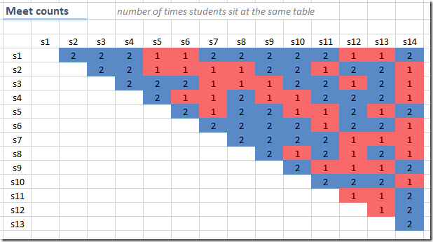
The new picture

image

shows only 2s and 3s (where again 3 means at least 3 months in between). I.e. we successfully removed all cases where student pairs sit at the same table with zero or one month in between.

References
  1. A more complex table seating problem: http://yetanothermathprogrammingconsultant.blogspot.com/2016/10/scheduling-business-dinners.html 
  2. A related problem: https://en.wikipedia.org/wiki/Kirkman's_schoolgirl_problem